Submarine Permafrost Maps Of The Russian Arctic. A Review

Alexander V. Vasiliev; Gleb E. Oblogov; Nataliia G. Belova

doi:10.24057/2071-9388-2025-3970

Submarine Permafrost Maps Of The Russian Arctic. A Review

Alexander V. Vasiliev, Gleb E. Oblogov, Nataliia G. Belova

https://doi.org/10.24057/2071-9388-2025-3970

Full Text:

PDF (Eng) HTML XML

Generate QR code

Contents

Scroll to:

Abstract

The article presents the results of digitizing the maps of submarine permafrost on the shelf of the Arctic seas of Russia. Submarine permafrost mapping relies heavily on expert knowledge because there is a lack of data regarding the structure and thickness of permafrost. Maps compiled by different authors vary significantly due to the use of different approaches, paleogeographic scenarios, ideas about the geological structure, evolution of shelf permafrost, sea level and climatic changes. The first maps were based on the analysis of shelf morphology and seawater temperature; they represent only the assumed boundaries of the submarine permafrost distribution. Later, the distribution of submarine permafrost was associated with neotectonic movements on the modern shelf. As the first drilling and seismoacoustic data were received, more detailed maps were compiled, and the discontinuous distribution of submarine permafrost was substantiated, especially in the Western Arctic. By now, a large amount of seismoacoustic and drilling data has been accumulated, which has made it possible to create new maps based on these data. In recent decades, methods of mathematical modeling the formation and evolution of submarine permafrost have been rapidly developed. Calculated maps of the distribution and depth of submarine permafrost top in the Russian Arctic have been compiled. For the first time, it has become possible to predict the rate of degradation of submarine permafrost under climate warming.

Keywords

Russian Arctic, shelf, submarine permafrost, maps

For citations:

Vasiliev A.V., Oblogov G.E., Belova N.G. Submarine Permafrost Maps Of The Russian Arctic. A Review. GEOGRAPHY, ENVIRONMENT, SUSTAINABILITY. 2025;18(3):107-117. https://doi.org/10.24057/2071-9388-2025-3970

INTRODUCTION

The study of submarine permafrost (SMP) is of interest in connection with the discovery of promising oil and gas fields on the shelf of the Russian Arctic and the development of the Northern Sea Route. Another important problem associated with SMP is the assessment of the role of permafrost in the formation of methane flows on the shelf of the Arctic seas (Bogoyavlensky et al. 2023a,b; Koshurnikov et al. 2020; Shakhova et al. 2015) and the overall impact of climate change on the Arctic environment.

Permafrost is formed when the shelf drains up during sea regression. During sea transgression, permafrost transitions to a subaqueous state, and its degradation occurs. New permafrost formation also occurs within currently developing marine accumulative forms (Grigoriev 1987).

The distribution and evolution of SMP in the Arctic have been the subject of many publications (Antipina et al. 1979; Zhigarev 1997; Kassens et al. 2000; Chen et al. 2022; Romanovskii et al. 1997; Romanovskii et al. 1999; Rokos et al. 2023 and many others).

Direct observations of the space distribution, thickness, state, and thermal regime of SMP are extremely limited. By 2024, only 17 boreholes had been drilled in the Barents and Kara Seas, which have exposed SMP. Drilling on the East Siberian Shelf commenced in 1953 (Grigoriev 1966) and has continued to the present day. Moreover, most of the boreholes are located in shallow coastal areas. At the same time, geophysical methods for studying SMP are increasingly advancing; among these, high-resolution seismic methods hold the greatest promise (Rekant and Vasiliev 2011; Kulikov et al. 2014; Overduin et al. 2015). Seismoacoustic profiling has become an almost mandatory task during marine expeditions. By now, a substantial number of seismoacoustic profiles have been completed in the Arctic seas. Methods of electrical exploration for the study of SMP are successfully developed by A.V. Koshurnikov (2023).

As our understanding of SMP evolves, attempts have been made to map its distribution, properties, and thickness. Due to limited data, most of the maps are based on expert assessments and reflect the authors’ perspectives on the potential distribution and conditions of the occurrence of SMP. Currently, there are several maps illustrating the potential distribution of subaqueous permafrost on the shelf based on the analysis of bottom temperature, bathymetry, and sea level rise data. Until recently, all these maps were available only in paper form. Some of these maps are currently unavailable for use, as they were only included in scientific and technical reports.

Recently, digital SMP maps compiled based on mathematical modeling of SMP formation and evolution have become increasingly widespread (Malakhova 2019; Smirnov et al. 2024; Nicolsky et al. 2012; Gavrilov et al. 2020; Malakhova and Eliseev 2020). The main drawback of such maps is an incomplete accounting of actual SMP data. The SMP parameters displayed on digital maps are calculated and can sometimes contradict even the limited factual information available. This issue is due to a lack of information, mainly on the boundary conditions used in mathematical models. Nonetheless, modeling the formation and evolution of SMP has resulted in a distinct and rapidly advancing field of SMP research.

This work is dedicated to the collection, processing, and analysis of approaches of published and archived maps of the SMP and the compilation of a GIS album, including SMP maps, some of which were previously inaccessible and unknown to researchers. Maps containing information about permafrost on the shelf of the Russian Arctic from published data, archives of the Institute of the Earth Cryosphere SB RAS, other institutes, and Rosgeolfond were processed. The purpose of the work is to ensure the availability of many published or unpublished (archived) maps of the SMP of the Russian Arctic.

MATERIALS AND METHODS

The QGIS geographic information system (GIS) was used. Today, it is among the most dynamically developing and functional desktop GIS applications. The main task was to digitize original paper maps. To work with GIS, it is essential to establish a correspondence between the internal coordinate system of the raster (graphic image) and the external (target) coordinate system used in the GIS project; in other words, it is necessary to perform raster referencing. Referencing consists of determining two pairs of coordinates for a certain number of points: coordinates in the internal coordinate system of the raster and coordinates in the target coordinate system. The reference points should be evenly distributed across the image (or at least the part used in the study) and not on the same line.

The Lambert Azimuthal Equal Area Projection (WGS 84/North Pole LAEA Russia) was selected as the coordinate system for the GIS project, as it is the most suitable for the cartographic representation of the Russian Arctic SMP. However, the created maps can easily be converted to any other projection. Additionally, one advantage of working in QGIS is the availability of base maps – coastline, hydrological network, and simplified topographic maps.

When digitizing the maps, we aimed to preserve the original legends as much as possible, as they reflect the authors’ approaches to constructing the maps and their content. However, in some cases, the legend had to be modified.

Here we offer the visual representation of the maps; if needed, GIS projects can be obtained from the publication’s authors.

RESULTS

By now, all available geocryological maps have been digitized. One of the first publications in 1972 was A.L. Chekhovsky’s forecast scheme for the distribution of the subaqueous cryolithozone in the Asian sector of the Arctic (Chekhovsky 1972). In conditions of insufficient information, the author, in fact, displayed the spatial distribution of water temperature in the Arctic seas, considering the shelf relief. The scheme does not illustrate subaqueous permafrost but rather the cryolithozone, understood as sediments that presumably have a negative temperature (Fig. 1). It should be noted that, when applied to the western sector of the Russian Arctic, the boundaries of the cryolithozone and the distribution area of subaqueous permafrost containing ice differ significantly from the modern data. A.L. Chekhovsky identified two types of cryolithozone in the Arctic seas: shelf cryolithozone, extending to a depth of 200 m, and oceanic cryolithozone, found at depths greater than 200–800 m. Within the shelf cryolithozone, with ground temperatures ranging from 0 to –1.8°C, areas with positive summer temperatures have been identified in the estuaries of large rivers. The oceanic cryolithozone, located to the north of the shelf, has temperatures of –0.7°C in the Atlantic sector of the Arctic and –0.35°C in the Pacific.

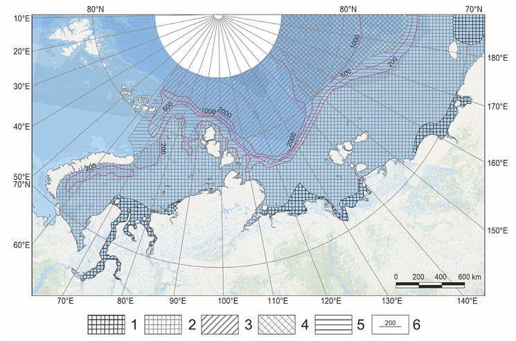
Fig. 1. Image of the forecast map of the distribution of cryolithozone in the Asian sector of the Arctic (Chekhovsky 1972). Legend: 1 – shelf cryolithozone, MAGT 0…-1°C with a positive summer water temperature; 2 – the same, but with a constant negative temperature; 3 – oceanic cryolithozone with MAGT -0.7°C; 4 – also with MAGT -0.35°C; 5 – unfrozen sediments with MAGT 0.6-2.0°C; 6 – isobaths, m

Later, the same approach to assessing the distribution of the shelf cryolithozone based on the spatial distribution of the temperature of the bottom water layer was used by L.A. Zhigarev in his monograph (1997). By the time the monograph was published, new data on seawater temperatures in the Arctic seas and, most importantly, the results of SMP studies in the coastal zones of the Laptev Sea, East Siberian Sea, and Chukchi Sea had been obtained. The monograph includes a schematic map of the cryolithozone in the Arctic seas of Russia. The map illustrates the boundaries of the distribution of alongshore permafrost (established and assumed), relict permafrost (established and assumed), seasonally frozen sediments (established), perennially and seasonally non-frozen sediments with temperatures below 0°C, cryotic sediments, and average annual isotherms (established and assumed). The author selected this classification of cryolithozone as a basis for identifying areas and regions that differ in the conditions of heat exchange between bottom sediments and seawater. The schematic map is created on a small scale, accompanied by an ineffective legend, making its practical use exceedingly challenging. The significant advantage of the schematic map was that it outlined the boundaries of the distribution of frozen rocks on the sea shelf of the Eastern Arctic. This schematic map has not been digitized.

In the 1950 and 1970s, the content was developed (Baranov 1960; 1972), and in 1977, the geocryological map of the USSR was published under the editorship of I. Ya. Baranov at a scale of 1:5,000,000. The map covers both the continental and shelf regions of the Russian Arctic. The construction of the marine part of the map was based on the concept of shelf drainage, freezing, and subsequent submersion and flooding of the shelf, along with the active involvement of tectonic movements (Fig. 2). The map for the first time reflected the boundaries of the SMP distribution in sufficient detail (Geocryo… 1977).

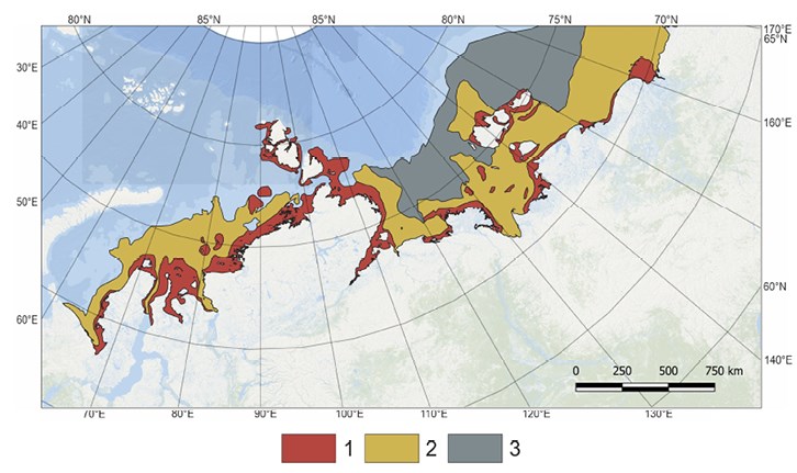
Fig. 2. Image of the marine part of the geocryological map of the USSR, edited by I. Baranov (1977). Legend: 1 – submarine permafrost in the inner part of the shelf, underlain by unfrozen saline sediments with a negative temperature; 2 – submarine permafrost in the outer part of the shelf partially thawed from above, underlain by unfrozen saline sediments with a negative temperature; 3 – unfrozen saline sediments with a negative temperature

Surprisingly, the boundaries of the SMP distribution in the Kara Sea on this map align closely with modern ones derived from drilling and seismic acoustic data.

As ideas about the SMP’s conditions, formation history, and evolution developed, more detailed maps began to be compiled using limited drilling data and high-resolution seismic data. One example is the map created by V.A. Soloviev for the Barents and Kara Seas (Fig. 3) (Soloviev et al. 1981).

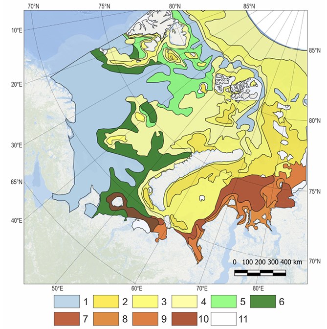
Fig. 3. Image of the SMP map of the Barents and Kara Seas (Soloviev et al. 1981). Legend: 1 – zone of positive temperatures; SMP: 2 –with a thickness of more than 50 m with cryopeg interlayers; 3 – with a thickness of 25-50 m with cryopeg interlayers; 4 – with a thickness of less than 25 m with cryopeg interlayers; 5 – seasonal submarine permafrost; 6 – episodically unfrozen area; 7 – area of sparse insular relict permafrost; 8 – insular relict permafrost with a thickness of less than 50 m; 9 – insular relict permafrost with a thickness of more than 100 m; 10 – insular relict permafrost beneath the episodically unfrozen zone; 11 – insular relict permafrost beneath the positive temperature zone

For the first time, the map reflects different SMP types and their continuity and provides estimates of their thickness. The legend uses the concepts of cryolithozone and frozen zone. Apparently, the term “cryolithozone” is used to designate negative-temperature sediments without ice inclusions, and the term “frozen zone” refers to frozen sediments that contain ice. The non-continuous nature of the SMP distribution in the Barents and Kara Seas is substantiated for the first time. Later, the map was improved, and became more detailed, and the legend was slightly changed.

The ideas about the SMP distribution developed by Ya.V. Neizvestnov and V.A. Solovyov were implemented in compiling the well-known and accessible Geocryological Map of the USSR at a scale of 1:2,500,000 (1996). When it was created, drilling and seismoacoustic research data from the Arctic seas were considered. However, the map’s legend in the part of the Arctic shelf turned out to be heavily overloaded and difficult to read. As a result, the practical utilization of the map for evaluating the distribution and conditions of SMP occurrence is quite challenging.

Later, the same authors tried to implement a qualitative assessment of the probability of the distribution of the SMP of different continuity – ranging from less probable to probable and then to more probable. When creating the map, in addition to considering the probability distribution of SMP, greater emphasis was placed on the morphology of the shelf and the temperature regime of the bottom layer of water. The map is characterized by a high level of spatial resolution, as the analysis of the distribution and conditions of occurrence of SMP was conducted for each sheet of the international sheet numbering on a scale of 1:1,000,000. Unfortunately, the map was not published and exists only in paper form in a report in the Rosgeolfond archive (Neizvestnov et al. 1991). The appearance of the map is shown in Fig. 4.

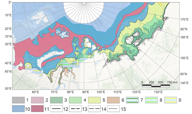
Fig. 4. Image of the forecast map of the cryolithozone of the shelf and islands of the Arctic seas of the USSR (Neizvestnov et al. 1991). Legend: 1 – continuous (newly formed) and relict permafrost zones turning into an island one; 2 – separate large massifs of frozen sediments within the island permafrost zone; 3 – island permafrost zone (more probabilistic distribution); 4 – island permafrost zone (probabilistic distribution); 5 – island permafrost zone (less probabilistic distribution); 6 – continuous relict permafrost zone under positive-temperature sediments; 7 – island relict permafrost zone under positive-temperature sediments (more probabilistic); 8 – island relict permafrost zone under positive-temperature sediments (probabilistic); 9 – island relict permafrost zone under positive-temperature sediments (less probabilistic); 10 – negative-temperature thawed non-frozen zone; 11 – positive-temperature zone; 12 – boundary of continuous permafrost, turning into an island permafrost; 13 – the boundary of the island permafrost; 14 – the boundary of the negative temperature thawed (not frozen) cryolithozone; 15 – the boundary of the intermediate island permafrost zone

In creating a circumpolar map of Arctic permafrost and ground ice, developed by an international team of researchers (Broun et al. 2001), the Russian part of the map is based on the previously published Geocryological Map of the USSR at a scale of 1:2,500,000 (1996). The production of a comprehensive circumpolar map depicting the distribution and thickness of SMP was undertaken at the initiative of the IPA as part of the European project NUNATARYUK. For the shelf permafrost of the Russian Arctic seas, the boundaries of the SMP distribution were clarified, and the map’s legend and content were considerably simplified. This map illustrates the spatial distribution of the SMP along with the thickness estimations of the added SMP. It is available on the GRID-Arenda website (Fig. 5). It should be noted that the permafrost thickness was estimated based on the depth of the 0°C isotherm. For the eastern sector of the Arctic, the thickness estimates are generally satisfactory and correspond to other calculations (Romanovskii et al. 1997; Nicolsky et al. 2012; Koshurnikov et al. 2020), while for the western sector, the values of the SMP thickness are extremely overestimated. Quaternary deposits on the shelf of the western Arctic are represented by a thick stratum of saline sandy-clayey soils of predominantly marine origin. The onset temperature for freezing and thawing can vary from 0 to –1.5°C, depending on the salt content and lithological composition. In this case, the SMP permafrost occupies only the upper portion of the section with temperatures below the phase transition temperature; beneath, it is underlain by non-frozen sediments.

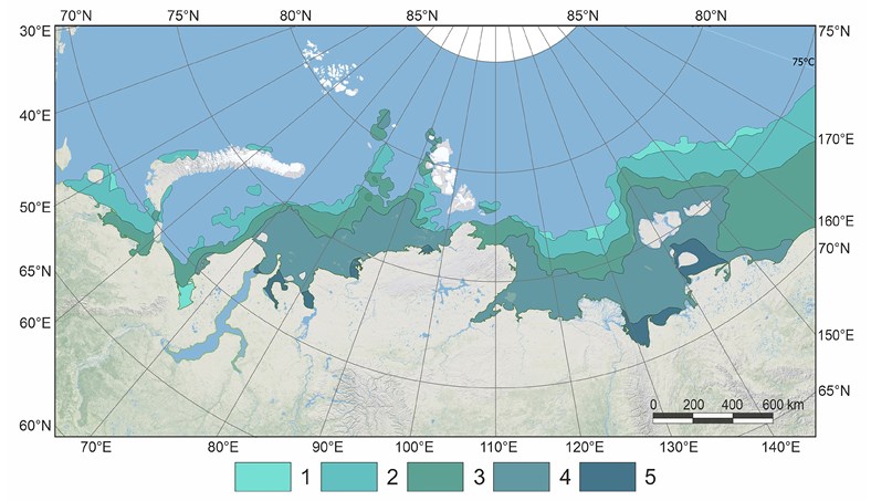
Fig. 5. Distribution and thickness of the submarine permafrost on the IPA map (Permafrost in the Northern Hemisphere 2020, based on Overduin et al. 2019). In the legend, the SMP thickness is as follows: 1 – 0-100 m; 2 – 100-300 m; 3 – 300-500 m; 4 – 500-700 m; 5 – 700-900 m

This same map was later used to model the submarine permafrost evolution from the Pleistocene to the Holocene. This was done to clarify the boundaries of the submarine permafrost’s distribution and to calculate its thickness and ice content (Overduin et al. 2019; Angelopoulos et al. 2020; Chen et al. 2022). Both the original map and the model may not only overestimate the SMP thickness but also exaggerate the boundaries of its distribution. In particular, in the Barents Sea, the SMP is present north of Kolguev Island. However, according to seismoacoustic profiling data, the SMP was not detected in this area, and the SMP boundary is situated south of what is indicated on the map. In the same way, the SMP map in the Kara Sea indicates a large submarine permafrost massif to the west of the Severnaya Zemlya archipelago. Detailed seismoacoustic observations revealed a widespread distribution of Late Pleistocene marginal moraines framing the ice shelf here (Polyak et al. 2008). Thus, there were no conditions for the SMP formation (Gusev et al. 2012).

With the acquisition of new drilling and seismoacoustic profiling data in the Kara and Barents Seas, it became possible to utilize this information not only to interpret the geological structure of the Quaternary strata but also to analyze the distribution of SMP. All available seismoacoustic profiling and drilling data were gathered and reinterpreted to search for SMP manifestations (Rekant and Vasiliev 2011). Thus, a database of manifestations and occurrence depths of SMP in these seas was developed, and a GIS-oriented map of their distribution was constructed (Fig. 6).

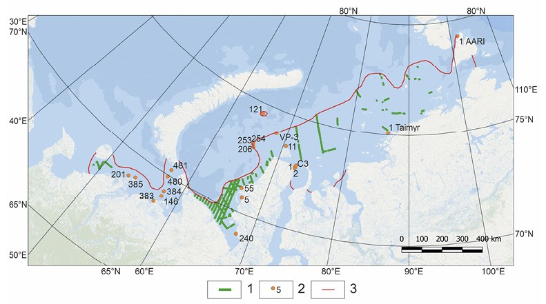
Fig. 6. Map of the distribution of submarine permafrost in the Barents and Kara Seas based on drilling and seismoacoustic profiling data (Rekant and Vasiliev 2011). Legend: 1 – seismoacoustic profiles; 2 – boreholes and their respective numbers; 3 – permafrost limit

The peculiarity of this map is the possibility of its continuous improvement and development as new seismoacoustic data become available and boreholes are drilled.

In 2025, V. Bogoyavlensky and co-authors published an article that provides a map of the SMP distribution in the Laptev Sea and the East Siberian Sea based on drilling data and, mainly, the results of deep seismic interpretation (Bogoyavlensky et al. 2025). The area of SMP distribution on this map is much smaller in the Laptev Sea, and SMP is completely absent in the East Siberian Sea. The authors explain these features of the SMP distribution through permafrost degradation, up to its complete thawing. This hypothesis contradicts all existing ideas about the distribution of SMP in the East Siberian seas. The Laptev and the East Siberian Seas shelves have a similar geological structure, a common paleogeographic history and a similar modern thermal regime of seawater. Therefore, the presence of permafrost in the Laptev Sea suggests that there are no reasons for it to completely thaw in the East Siberian Sea. Most likely, the source of the discrepancy is the incorrect interpretation of deep seismic data.

A detailed map of the distribution of SMP in the Russian Arctic was created at VNIIokeangeologiya (Shcherbakov et al. 2018). It considered all the drilling data and the results of our own seismoacoustic profiling in both the western and eastern sectors of the Arctic that were available at that time. The map reveals for the first time the spatial distribution of SMPs in various percentages of the permafrost area and offers more substantiated estimates of the thickness and temperature of frozen sediments than previous assessments. (Fig. 7). The water area of the Russian Arctic seas is divided into zones according to cryolithozone types. The boundaries of the SMP itself and non-frozen sediments are plotted. The VNIIokeangeologiya map illustrates the distribution of SMP in the seas of the Eastern Arctic with much greater detail. For the first time, potential new SMP formation areas are indicated on the shelf of the Arctic seas, based on the presence of bottom temperatures that fall below the phase transition temperature. However, according to direct observations (Dubrovin 2015; Rokos et al. 2023), a decrease in bottom temperatures only leads to the formation of frozen crusts with a thickness of no more than 0.2...0.5 m in the near-surface part of the section, which completely thaws during the summer season. Stable permafrost formation under current conditions is impossible in any area of the Arctic shelf.

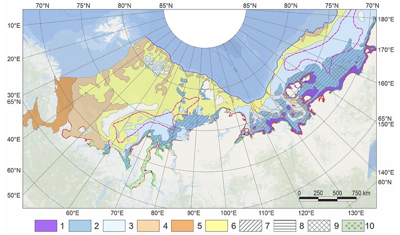
Fig. 7. An image of the SMP map of the Russian Arctic, VNIIokeangeologiya (Shcherbakov et al. 2018). Legend: 1 – relict and newly formed continuous, turning into an island, frozen submarine cryolithozone; 2 – island relict submarine frozen zone; 3 – rare island submarine frozen zone; 4 – negative-temperature frozen submarine cryolithozone with sediments temperature of 0…-1°C; 5 – positive-temperature zone; 6 – negative-temperature unfrozen submarine cryolithozone with sediment temperature of -1…-2°C; 7-9 –permafrost thickness: 7 – from 0 to 100 m, 8 – from 100 to 200 m, 9 – more than 200 m; 10 – submarine taliks; 11 – geocryological boundaries; 12 – zones of tectonic faults with endogenous through submarine taliks with the base of the permafrost layer raised by 100-200 m; 13 – supposed areas of modern permafrost formation; 14 – accumulative coasts; 15 – thermoerosional coasts; 16 – shelf boundary

In 2023, the Arctic Permafrost Atlas was published, which contains several maps characterizing the SMP (Westerveld et al. 2023). As an example, Fig. 8 shows a fragment of the distribution map of the Russian Arctic SMP based on modeling. In fact, the album repeats the maps (Fig. 5) given in the publications (Overduin et al. 2019; Angelopoulos et al. 2020). Contradictions regarding the distribution boundary of the SMP and its thickness remained unresolved when the atlas was published.

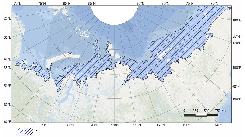
Fig. 8. Image of the Russian Arctic SMP distribution map according to (Westerveld et al. 2023). Legend: 1 – SMP distribution area

A promising method for studying the SMP using electrical exploration is being developed by A.V. Koshurnikov. Based on marine profiles in the Arctic seas of Russia, he showed that the specific electrical resistance of frozen strata and potential gas hydrates under permafrost are close to each other. The proximity does not allow them to be separated on the profiles. A map of the distribution of the SMP and the total thickness of SMP and gas hydrates has been developed (Koshurnikov, 2023). When digitizing the map, the legend was simplified (Fig. 9), and a different color scheme was used. The areas of distribution of the SMP and the total thickness of SMP and gas hydrates for the Barents and Kara Seas shown on the map differ greatly from other maps. The author explains these differences by the widespread development of saline Quaternary deposits on the shelf of the Western Arctic, which greatly complicates the interpretation of field observations.

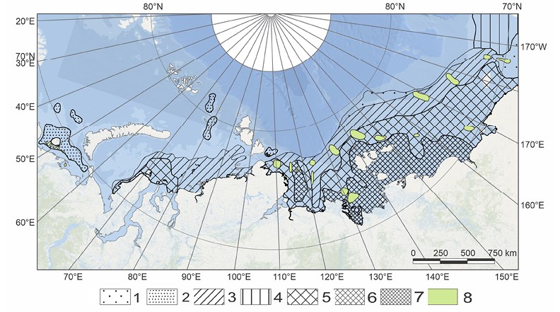
Fig. 9. An image of the SMP and gas hydrate distribution and total thickness in the Russian Arctic (Koshurnikov 2023). Legend: 1-7 – thickness of the cryogenic strata, m: 1 – 100-200, 2 – 200-300, 3 – 300-400, 4 – 400-500, 5 – 500-600, 6 – 800-900, 7 – more than 1000; 8 – high-temperature cryogenic strata

Geoelectric surveys by magnetotelluric and transient electromagnetic methods have good prospects for subaqueous permafrost mapping (Yakovlev et al. 2018). The application of the method in the Khatanga Gulf has shown its effectiveness in determining the depth of the SMP top.

In recent decades, the construction of submarine permafrost maps based on mathematical modeling has been actively developing. Permafrost formation is considered a result of a long geological history of shelf development, with periodic stages of cooling and warming, transgressions, and regressions in the Arctic Ocean. As a rule, a heat exchange model based on the solution of the Stefan problem is used here. The primary issue with this modeling is to consider the characteristics of the geological structure of the Arctic shelf, as well as the composition, ice content, salinity, and temperature of phase transitions. The upper boundary conditions are established according to the chosen paleogeographic scenarios. In this case, specific paleotemperatures of the air are often assigned based on indirect data. The temperature on the Earth’s surface is set equal to the air temperature. However, actual observations of modern air temperatures (MAAT) and permafrost temperatures (MAGT) show that the ratio of MAGT and MAAT ranges from 0.1 to 1.0 depending on the landscape conditions that determine the heat exchange at the surface. The average ratio between modern MAGT and MAAT for the western sector of the Russian Arctic is about 0.7 (Malkova et al. 2022).

An example of SMP maps constructed through mathematical modeling can be the map of the distribution and thickness of the SMP in the Kara Sea (Gavrilov et al. 2020) (Fig. 10).

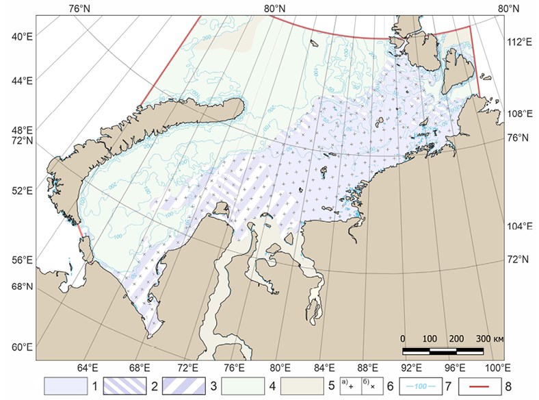
Fig. 10. Image of the submarine permafrost distribution and thickness map constructed based on mathematical modeling (Gavrilov et al. 2020). Legend: 1 – continuous SMP with a thickness of 100-300 m; 2 – discontinuous massive island and island SMP with a thickness of 0-100 m; 3 – island SMP with a thickness of 0-100 m; 4 – non-frozen cryotic sediments; 5 – thawed sediments; 6 – depth of the SMP top: a – 0-30 m, b – 25-50 m or more: 7 – isobaths; 8 – boundaries of the study area

When creating the map, the authors considered the 125 Kyr history of the Kara Sea shelf development. The model takes into account not only the change in sea level during the Late Pleistocene but also the eustatic uplift of the dried shelf surface during the postglacial transgression. Since the model contains several uncertainties in the properties of freezing bottom sediments, the temperature of the bottom water layer, paleoclimate, etc., the authors adopted broad ranges of the SMP thickness shown on the map in the legend. This enabled the identification of areas with sharply contrasting calculated thickness values. The map highlights a region with a SMP thickness of 100-300 m. However, A. Portnov showed that under the most severe climatic conditions of the Last Glacial Maximum in the Kara Sea, the submarine permafrost thickness cannot exceed 270 m (Portnov et al. 2014). Considering the SMP degradation from above and below, its maximum thickness cannot exceed 200-250 m. The area of SMP distribution in the southern part of the Kara Sea is underestimated when compared to seismoacoustic profiling data, whereas it is overestimated in the central and northern parts of the sea. Later, an analogous map was compiled for the Laptev Sea (Gavrilov et al. 2024).

More efficient but also more complex modeling of the SMP is being developed in the Institute of Computational Mathematics and Mathematical Geophysics SB RAS (Malakhova 2019; Malakhova et al. 2020; Malakhova 2023; Malakhova and Eliseev 2023). This model uses both climate and heat exchange models in the Arctic Ocean. This approach allowed V. Malakhova, for the first time, to not only establish the modeled boundaries of the distribution of the SMP and its thickness (Fig. 11) but also to assess the current and projected trends of its degradation in the Russian Arctic. Under the RSP scenario of 8.5, the average rates of SMP degradation were 1-2 cm per year for 1950-2015, 5 cm per year for 2015-2100, and 10 cm per year for 2100-2300.

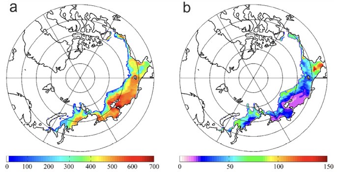
Fig. 11. Modeled submarine permafrost in the XX century. (a) The depth of the lower subsea permafrost boundary (in m). (b) The depth of the upper submarine permafrost boundary (in m) (Malakhova 2023)

The map was not digitized due to its small scale.

Yu. Smirnov and co-authors (Smirnov et al. 2024) modeled the SMP, taking into account the climate zonality and spatial distribution of salinity in the seas of the Russian Arctic.

The boundaries of the distribution of the SMP on the map by Yu. Smirnov et al. for the central and southern Kara Sea demonstrate good agreement with those previously established based on seismoacoustic profiling and drilling data on the shelf (Rekant and Vasiliev 2011; Overduin et al. 2019), but for the Barents Sea, the area of the SMP distribution is clearly underestimated (see Fig. 6). Furthermore, in both seas, the depth of the SMP top is significantly underestimated. This is attributed to both the model’s imperfections and the uncertainties regarding the characteristics of the soils on the shelf and the boundary conditions.

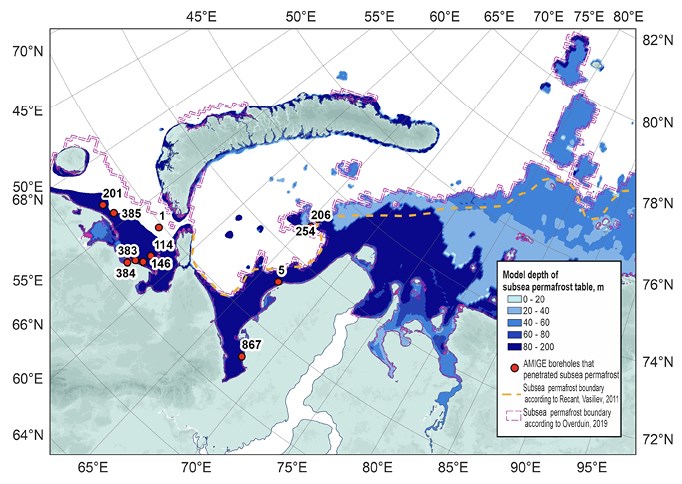
Fig. 12. Distribution and depth of the top of the submarine permafrost of the Kara and Barents Seas (Smirnov et al. 2024)

CONCLUSIONS

The conducted studies made it possible to ensure the availability of many published and unpublished (archive) maps of the Russian Arctic submarine permafrost. All maps were digitized and integrated into a single GIS format, enabling comparison. The review indicates that as the ideas about the distribution, conditions of occurrence, and thickness of the submarine permafrost developed, the content of the maps also changed.

The first maps were based on an analysis of the morphology of the Arctic shelf and seawater temperature. They only approximately reflected the boundaries of the spatial distribution of the sea and ocean cryolithozone, as well as the temperature of the bottom sediments.

I. Baranov developed ideas about the significant influence of neotectonics on the SMP’s distribution and conditions of occurrence. A more or less detailed geocryological map of the continental zone and shelf of the Russian Arctic was compiled.

Since the early 1980s, the first factual data on SMP in the Barents and Kara Seas have been obtained based on offshore drilling and imperfect geophysical data. The concept of a predominantly discontinuous massive island and the island nature of SMP distribution in the Western Arctic has been established. In contrast, shallow drilling data from the Eastern Arctic shelf have provided a basis for the assumption of continuous, less frequently intermittent SMP in this region.

The development of methods and hardware for seismoacoustic profiling has become a powerful tool in SMP studying. Prognostic maps of SMP distribution were compiled to assess the probability of the occurrence of different types of continuity. The boundaries of SMP distribution were defined, and by the 1990s, estimates of its thickness appeared.

As seismoacoustic methods evolved and data on the manifestation of SMP was accumulated, including ongoing drilling, maps were constructed that substantiated the boundaries of SMP distribution and the depth of the top with factual data.

A major step in the study of shelf permafrost was the development of methods for mathematical modeling of the formation and evolution of SMP. Several maps were created reflecting the distribution and conditions of the SMP occurrence. These maps are detailed, but uncertainty in determining the properties of the sediments on the shelf and, most importantly, the boundary conditions leads to significant deviations in the estimates of the thickness and depth of the SMP top. Improvement of the models made it possible to develop methods for predicting the current and further degradation of the SMP under global warming and changes in the hydrology of the Arctic seas.

Digitization of the maps of SMP of the Russian Arctic shelf, which were created based on various approaches, and in different periods, and the formation of an album of GIS-oriented maps, can be used to compile more detailed maps of the cryolithozone of the shelf and for comparison of modeling results and actual data.

References

1. Angelopoulos M., Overduin P.P., Miesner F., Grigoriev M.N., Vasiliev A.A. (2020). Recent advances in the study of Arctic submarine permafrost. Permafrost and Periglac.Process., 31, 442-453. DOI: 10.1002/ppp.2061.

2. Antipina Z.N., Are F.E., Voichenko V.V., Molochushkin E.N. (1979). Cryolithozone of the Arctic shelf of Asia. In: Late Quaternary history and sedimentogenesis of marginal and internal seas. Moscow, Russia: Nauka, pp. 183-189 (in Russian).

3. Baranov I.Ya. (1960). Geocryological map of the USSR at a scale of 1:10,000,000 (explanatory note). Moscow: Znanie, 48 p. (in Russian).

4. Baranov I.Ya. (1972). Geocryological (permafrost) map of the USSR at a scale of 1:5,000,000. Proceedings of the scientific All-Union conference on permafrost science. Moscow: Moscow State University Press, pp. 118-131 (in Russian).

5. Bogoyavlensky V., Kishankov A., Kazanin A. (2023a). Evidence of large-scale absence of frozen ground and gas hydrates in the northern part of the East Siberian Arctic shelf (Laptev and East Siberian seas). Marine and Petroleum Geology, 148, 106050, pp. 1-15.

6. Bogoyavlensky V.I., Kishankov A.V., Kazanin A.G. (2023b). Distribution of subaqueous permafrost in the Laptev Sea according to seismic exploration data using the refraction wave method. Arctic: ecology and economics, 13(4), pp. 501-515, DOI: 10.25283/2223-4594-2023-4-501-515. (in Russian).

7. Bogoyavlensky V. I., Kishankov A. V., Kazanin A. G. (2025). New information on subsea frozen ground in the Laptev and East Siberian seas based on seismic data. Doklady Earth Sciences, 521(11). DOI: 10.1134/S1028334X24605583.

8. Brown J., Ferrians O.J.J., Heginbottom J.A. and Melnikov E.S. (2001). Circum-Arctic map of permafrost and ground-ice conditions. Washington, DC: US Geological Survey in Cooperation with the Circum-Pacific Council for Energy and Mineral Resources. DOI: 10.3133/cp45.

9. Chekhovsky A.L. (1972). On the distribution of permafrost rocks under the shelf of the Kara Sea. Proceedings of the PNIIIS Gosstroy of the USSR. Moscow, vol. 18, pp. 100-110 (in Russian).

10. Chen Y., Li Q., Wen M., Wang Y., Duan W. (2022). Analytical and Numerical Analyzes on Vertical Site Responses of Submarine Permafrost in the Polar Ocean. Energies, 15, 5941. DOI: 10.3390/en15165941.

11. Dubrovin V.A. (2015). Results of drilling boreholes on the shelf of the Kara Sea in the area of the Marre-Sale geocryological station and the near future of its study. Proceedings of the International Conference “Arctic, Subarctic: mosaic, contrast, variability of the cryosphere”, July 2–5, 2015, Tyumen: Epoch, pp. 109–111 (in Russian).

12. Gavrilov A.V., Malakhova V.V., Pizhankova E.I., Popova A.A., Buldovich S.N., Rolsklyakov A.G., Khilemonyuk V.Z. (2024). The state of the Arctic shelf cryolithozone and requirements for the necessary modern factual data for geocryological mapping. Proceedings of the VII International Geological and Geophysical Conference GeoEurasia 2024, vol. I, Tver: Poli Press LLC, pp. 372-378 (in Russian).

13. Gavrilov A., Pavlov V., Fridenberg A., Boldyrev M., Khilimonyuk V., Pizhankova E., Buldovich S., Kosevich N., Alyautdinov A., Ogienko M., Roslyakov A., Cherbunina M., and Ospennikov E. (2020). The current state and 125 kyr history of permafrost on the Kara Sea shelf: modeling constraints. The Cryosphere, 14, 1857–1873, DOI: 10.5194/tc-14-1857-2020.

14. Geocryological map of the USSR (1977). Edited by I.Ya. Baranov. Moscow, Main Directorate of Geodesy and Cartography under the Council of Ministers of the USSR.

15. Geocryological map of the USSR, scale 1:2,500,000 (1996). Edited by E.D. Ershov. Vinnitsa Cartographic Factory.

16. Grigoriev N.F. (1966). Permafrost of the Coastal zone of Yakutia. Moscow: Nauka, 180 p. (in Russian).

17. Grigoriev N.F. (1987). Cryolithozone of the coastal part of Western Yamal. Yakutsk: Publishing House of the Institute of the Sea of the Siberian Branch of the Russian Academy of Sciences, 111 p. (in Russian).

18. Gusev E.A., Kostin D.A., Markina N.V., Rekant P.V., Sharin V.V., Dorechkina D.E., Zarkhidze D.V. (2012). Problems of mapping and genetic interpretation of Quaternary deposits of the Arctic shelf of Russia (based on materials of GGK-1000/3). Regional Geology and Metallogeny, 50, pp. 5-14. (in Russian).

19. Kassens H. Bauch H., Drachev S., Gierlichs A., Niessen F., Taldenkova E., Roudoy A., Thiede J., Wessels M. (2000). The Transdrift VIII expedition to the Laptev Sea: the shelf drilling campaign of «Laptev Sea System 2000». Terra Nostra. No. 8, p. 39-40.

20. Koshurnikov A.V. (2023) Permafrost of the shelf of the Russian Arctic seas (based on geophysical research data). Abstract of Doctoral thesis. Moscow, Moscow University Press, 45 p.

21. Koshurnikov A.V., Tumskoy V.E., Skosar V.V., Efimov Ya.O., Kornishin K.A., Bekker A.T., Piskunov Yu.G., Tsimbelman N.Ya., Kosmach D.A. (2020). Submarine permafrost in the Laptev Sea. Intern. J. of Offshore and Polar Engineering, 30(1), pp. 86-93. DOI: 10.17736/ijope.2020.jc783.

22. Kulikov S.N., Rokos S.I., Tulapin A.V. (2014). On the criteria for identifying permafrost rock massifs in the Pechora Sea and southwestern Kara Sea on time sections of seismoacoustic profiling. Engineering Geophysics, 2014. Conference Proceedings. April 21-25, 2014. Gelendzhik, pp. 1-8. (in Russian).

23. Malakhova V. (2023). Modeling of the Arctic subsea permafrost thawing under possible climate warming. Proc. SPIE 12780, 29th International Symposium on Atmospheric and Ocean Optics: Atmospheric Physics, 127804U (17 October 2023). DOI: 10.1117/12.2688510.

24. Malakhova V.V. (2019). Subaqueous permafrost of the Arctic shelf: assessment of thickness and area of distribution. Proceedings of the XIII Siberian Conference and School of Young Scientists on Climate and Environmental Monitoring. October 15-19, 2019, Tomsk. (in Russian)

25. Malakhova V.V., Eliseev A.V. (2023). A Relationship between Changes of Surface Air and Sea Floor Temperatures at the Arctic Shelf from the Coupled Models Intercomparison Project, Phase 6 Data. Atmosphere, V. 14. P. 1024. DOI: 10.3390/atmos14061024.

26. Malakhova V.V., Eliseev V.A. (2020). Salt diffusion effect on the submarine permafrost state and distribution as well as on the stability zone of methane hydrates on the Laptev Sea shelf. Ice and Snow, 60, 533–546, (in Russian with English summary), DOI: 10.31857/S2076673420040058.

27. Malkova G., Drozdov D., Vasiliev A. et al. (2022). Spatial and Temporal Variability of Permafrost in the Western Part of the Russian Arctic. Energies, 15, 2311. DOI: 10.3390/en15072311.

28. Neizvestnov Ya.V., Soloviev V.A. et al. (1991). Forecast map of cryolithozone types of the shelf and islands of the Arctic seas of the USSR at a scale of 1:5,000,000. Scientific and technical report. Moscow, Rosgeolfond, No. 360606. (in Russian).

29. Nicolsky D.J., Romanovsky V.E., Romanovskii N.N., Kholodov A.L., Shakhova N.E., Semiletov I.P. (2012). Modeling Sub-Sea Permafrost in the East Siberian Arctic Shelf: The Laptev Sea Region. J. Geophys. Res. Earth Surf., 117, 1–22. DOI: 10.1029/2012JF002358.

30. Overduin P.P., Haberland C., Ryberg T., Kneier F., Jacobi T., Grigoriev M.N. and Ohrnberger M. (2015). Submarine permafrost depth from 385 ambient seismic noise. Geophysical Research Letters, 42, 7581–7588. DOI: 10.1002/2015GL065409.

31. Overduin P.P., Schneider von Deimling T., Miesner F., Grigoriev M.N., Ruppel C., Vasiliev A., Lantuit H., Juhls B. and Westermann S. (2019). Submarine permafrost map in the Arctic modeled using 1-D transient heat flux (SuPerMAP). Journal of Geophysical Research: Oceans, 124, 6, pp. 3490-3507. DOI: 10.1029/2018JC014675.

32. Permafrost in the Northern Hemisphere (2020). [online] Produced as a part of Nunataryuk research project. Cartographer: GRID-Arendal/Nunataryuk. Available at: https://www.grida.no/resources/13519 [Accessed 25 Mar. 2025].

33. Polyak L., Niessen F., Gataullin V., Gainanov V. (2008). The eastern extent of the Barents–Kara ice sheet during the Last Glacial Maximum based on seismic-reflection data from the eastern Kara Sea. Polar Research, 27, pp. 162–174. DOI: 10.1111/j.1751-8369.2008.00061.

34. Portnov A., Mienert J., Serov P. (2014). Modeling the evolution of climate-sensitive Arctic subsea permafrost in regions of extensive gas expulsion at the West Yamal shelf. Journal of Geophysical Research: Biogeosciences, 119 (11), pp. 2082-2094. DOI: 10.1002/2014JG002685.

35. Rekant P.V. and Vasiliev A.A. (2011). Offshore permafrost in the Kara Sea. Earth’s Cryosphere, 15(4), pp. 60-62.

36. Rokos S.I., Kostin D.A., Tulapin A.V., Kulikov S.N., Dlugach A.G. (2023). Frozen and cryotic soils in the Baydarata Bay area. Earth’s Cryosphere, 27(5), pp. 3–13.

37. Romanovskii N.N., Gavrilov A.V., Pustovoit G.V., Kholodov A.L., et al. (1997). Off-shore permafrost distribution on the Laptev Sea shelf. Earth’s Cryosphere, 1(3), pp. 9-18. (in Russian with English summary).

38. Romanovskii N.N., Kholodov А.L., Gavrilov А.V., Tumskoy V.Е., Hubberten Н.W., Kassens Н. (1999) Ice-bonded permafrost thickness in the eastern part of the Laptev Sea shelf (results of computer modeling). Earth’s Cryosphere, 3(2), pp. 22-32. (in Russian with English summary).

39. Shakhova N., Semiletov I., Sergienko V., Lobkovsky L., Yusupov V., Salyuk A., Salomatin A., Chernykh D., Kosmach D., Panteleev G., Nikolsky D., Samarkin V., Joye S., Charkin A., Dudarev O., Meluzov A., and Gustafsson O. (2015). The East Siberian Arctic Shelf: towards further assessment of permafrost-related methane fluxes and the role of sea ice. Phil. Trans. R. Soc. A., vol. 373, p. 2052. DOI: 10.1098/rsta.2014.0451.

40. Shcherbakov V.A., Ivanova V.V., Slinchenkov V.I. et al. (2018). Geocryological map of the marginal seas of the Arctic Ocean of the Arctic Zone of the Russian Federation at a scale of 1:5,000,000.. Explanatory note. St. Petersburg, FGBU «VNIIOkeangeologiya», 52 p. (in Russian).

41. Smirnov Yu.Yu., Matveeva T.V., Shchur N.A., Shchur A.A., Bochkarev A.V. (2024). Numerical modeling of subaqueous permafrost on the Eurasian Arctic shelf taking into account the zonality of the modern climate. Earth’s Cryosphere, 28(5), pp. 38-59. DOI: 10.15372/kz20240504. (in Russian with English summary).

42. Soloviev V.A., Ginsburg G.D., Mikhalyuk Yu.N., Stanishcheva O.N., Telepnev E.V. (1981). Assessment of permafrost-geothermal conditions of the Barents-Kara shelf (report on topic 709). Leningrad, VNIIOkeangeologiya, 175 p., 12 graphs. appendix. (in Russian).

43. Westerveld L., Kurvits T., Schoolmeester T. et al. (2023) NUNATARYUK consortium. 2023. Arctic Permafrost Atlas. GRID- Arendal. DOI: 10.61523/KPJI4549.

44. Yakovlev D.V., Yakovlev A.G., Valyasina O.A. (2018). Permafrost study in the northern margin of the Siberian platform based on regional geoelectric survey data. Earth’s Cryosphere, 22(5), pp. 67-84. DOI: 10.21782/EC2541-9994-2018-5(67-84)

45. Zhigarev L.A. (1997). Oceanic cryolithozone. Moscow: Moscow State University, 320 p. (in Russian).