Contents
Scroll to:
https://doi.org/10.24057/2071-9388-2025-3735
Scroll to:
This paper provides a review and comparison of the methods for assessing trends in the dynamics of alpine treeline (ATL) in high mountains are presented in. The methods analyzed are contemporary, traditionally used (dendrochronological and paleocarpological methods, retrospective analysis of historical photographs and geodetic surveying, and multi-temporal aerial photography), and innovative ones developed in recent decades (semi-automatic and automatic methods of interpretation of high- and medium-resolution space imagery and methods of space imagery interpretation using different techniques, such as classification, segmentation, vegetation index analysis, and machine learning algorithms). Different interpretations of the concept of 'alpine treeline', which is currently established in geobotany and landscape sciences, are discussed. The attention to ATL dynamics is caused by global climate change's widespread forest increase and the decline in high mountain pastures. The ATL phenomenon's geographic map is condensed and displayed. There is an overview of the experience with different methods in varying mountain regions around the world. Each method is described in terms of its spatial scale, coverage, advantages, labor intensity, complexity, and limitations. It is shown that The effectiveness of the methods mainly depends on two key factors: the size of the area being studied and the time period over which changes are observed. The problem that still limits the use of remote sensing data is the contradiction between the accuracy of measurements and the coverage of the territories involved. To solve this problem, we suggest using a mix of methods that involve automatically classifying medium-resolution space images. This will be done by training on data collected from both fieldwork and lab experiments using different techniques.
Purekhovsky A.G., Gunya A.N., Kolbowsky E.Yu., Aleinikov A.A. Methods Of Studying The Alpine Treeline: A Systematic Review. GEOGRAPHY, ENVIRONMENT, SUSTAINABILITY. 2025;18(1):105-116. https://doi.org/10.24057/2071-9388-2025-3735
In mountainous areas, where the growing conditions for tree and shrub species become critically unfavorable, a treeline (alpine treeline [ATL]) is an important integral feature accessible for recording and measurement by both visual and instrumental methods. A relatively narrow ecotone (sometimes several meters but more often the first dozens of meters) between the ‘subalpine’ forest with a more or less closed forest canopy and open herbaceous vegetation is clearly visible in the upper mountain belt through remote sensing of the Earth. At the same time, a treeline is very sensitive to average, long-term trends in climate change; both of these circumstances make the conventional ATL a popular object of research to monitor the transformation of high-mountain landscapes worldwide (Steinbauer et al. 2016).
There is no doubt that the climate plays an important role in the dynamics of the ATL (Pearson and Dawson 2003). Microclimatic research at the forest edge revealed that the nature of forest growth was decisively influenced by temperature conditions: the sum of active temperatures in a vegetation period limits tree growth, and winter temperatures play a key role in the survival of young trees and the likelihood of damage to adult specimens (Chen et al. 2011). Changes in air and soil temperature (especially in spring), as well as increases or decreases in precipitation, lead to weaker or stronger impacts of climatic factors on all phases of the life cycle and vegetation of plants. In turn, this affects the germination and survival of undergrowth and predetermines the tree growth rate and mortality of adult trees at the boundaries of their distribution areas. However, the recorded shift and transformation of forest boundaries cannot be explained solely by temperature and moisture exchange factors; this would be an oversimplification. When observing both the upper (altitude) forest boundary in the mountains and the northern (latitudinal) forest boundary, it becomes clear that the changes in these two global ecotones are caused by complex cause-and-effect relationships among various landscape components, primarily climate and vegetation, as well as mesorelief, soil type, soil moisture dynamics, plant succession, and previous (historical) and current economic use (i.e. anthropogenic load; Lenoir et al. 2009).
In the mountains, the geomorphometric parameters of relief (slope gradient, aspect, plane curvature and profile curvature) play a particularly important role in the formation of heat and moisture exchange conditions and, consequently, in the differentiation of landscape sites. The macrorelief of the mountains (inter- and intra-mountain depressions, long and deeply rugged ravines and ridges) modifies regional climatic regimes and generally causes significant differences in ATL localization. At the local level, the microrelief (slope, peak and saddle, ridge and spur surfaces) predetermines the existence of harsh (windward, dry, extremely arid or ‘cold’) and favorable (humid, warm and wind-shadowed) habitats. The latter can form a kind of refugium, where both the actual position of the ATL and its response to climatic fluctuations will differ from the general regional one. These factors make a contribution to the different scales of localization and transformation of ATL, the latter being a phenomenon of the landscape structure of mountains (Morley et al. 2018).
High-mountain forests are important carbon accumulation and sequestration zones. They conserve soils and groundwater basins that feed a significant share of the world's population. Studying their changes is necessary for understanding the consequences of the loss of ecosystem services, especially at a time of sharp climate fluctuations associated with global warming (Devos et al. 2022). Current climate change scenarios predict a 0.3°C–4.8°C increase in the average global temperature by 2100 compared to the 1985–2005 average (IPCC 2013). Therefore, there is every reason to expect significant shifts in the geographic distribution of a large number of tree species, for which the change in heat and water availability may affect range expansion, shrinkage, or fragmentation. Mountain areas will experience larger increases in seasonal temperatures compared to other parts of the world, making them important indicators of global climate change effects (Calvin et al. 2023). However, the cause-and-effect relationships between the climate and the ATL are still poorly understood. ATL dynamics manifest themselves differently in various mountain regions; explaining these differences by historical and/or current patterns of nature management is significantly complicated.
The long-term isolation of mountain forests and fragmentation of habitats have resulted in exceptionally large numbers of endemic and rare plant and animal species inhabiting mountain areas. Any changes in the distribution of mountain forests caused by either climate change or anthropogenic load affect the biodiversity of the entire region significantly. Studies of forest distribution in the mountains are relevant for assessing the contribution of global climate change to the dynamics of ecosystems and landscapes. Our research focuses on organizing the ways to study the ATL and identifying the problems with these methods by looking at recent scientific articles and our own research data.
The studies of the state and dynamics of the ATL date back to the late 19th–early 20th centuries, when they were based primarily on visual comparison methods and analyzing various kinds of historical evidence (e.g. oral reports, old maps or travelers’ texts). This, indeed, provided very rough estimates. Although such estimates were not systematic, they allowed for drawing some conclusions about the key position factors and ATL dynamics. More specialized studies of the treeline began in the 1930s, alongside the study of the physiological response of trees and undergrowth under critical environmental conditions in the mountains (Holtmeier and Broll 2019). Researchers also conducted both in situ and in vivo experimental studies (Däniker 1923; Steiner 1935).
The catastrophic avalanches in the European Alps in the middle of the 20th century, caused by the super snowy winters of 1951–1954 gave new impetus to fundamental and applied treeline research. In Austria and Switzerland, a detailed analysis of the physiological response of trees located in the marginal zone of their habitat to climatic parameters and human economic impact was performed. These results made it possible to lay the scientific foundations for mountain forest management, including, most importantly, the practices of forest restoration (Holtmeier 2010).
After it was concluded that the modern treeline tends to shift upwards in mountain systems and to northern latitudes on the plain due to climate change, this phenomenon attracted much attention from researchers in the late 20th century. Since the 1990s, the number of publications on this topic has increased rapidly (by about 90%) due to the availability of remote sensing data and the possibility of developing geospatial models (Holtmeier and Broll 2019).
Forest boundary studies by geographers, landscape ecologists, foresters, and forest geobotanists have become focused on the analysis of the configuration of forest area boundaries under the influence of both natural (abiotic and biotic) and anthropogenic factors. The diversity of natural conditions and the multiplicity of invariants of economic impact (including historical and inherited variants) have generated significant inconsistencies in the generalizations and interpretations of results, especially when attempting to use models and extrapolate local data to macro-regional and global levels.
The development of remote sensing methods in recent decades (aerial imagery, orthophotoplanes, medium- and high-resolution satellite images and LiDAR photography), along with geostatistical analysis, initiated building local spatiotemporal models of forest ecosystems. These studies have contributed to a more comprehensive understanding of the driving factors of ATL changes, including the influence of the entire complex of landscape conditions (lithological, geomorphological, soil, hydrological, etc.) on spatio-temporal patterns of ATL dynamics and associated ecological processes at regional, zonal, and global scales (Morley et al. 2018).
A particular problem in studying the dynamics of mountain landscapes has always been their poor accessibility. Therefore, the model territories of these studies are small in area and unevenly distributed across different mountain systems. As a rule, long-term studies (monitoring) are conducted at the same place (e.g. at university sites); this allows for considering already accumulated field material (geobotanical descriptions, large-scale landscape maps and photographs). Meanwhile, specialists may ignore areas near or far from such sites. Therefore, a significant number of the already completed field studies, when generalized at the global (and even macroregional) scales, represent a set of randomly distributed ‘points’ (Fig. 1). Even if these studies are supported by geospatial models obtained using modern remote sensing processing methods, the available and even pooled information does not yet allow one to build a reliable overall picture of the localization and transformation of the upper boundary of mountain forests on different continents of the planet.
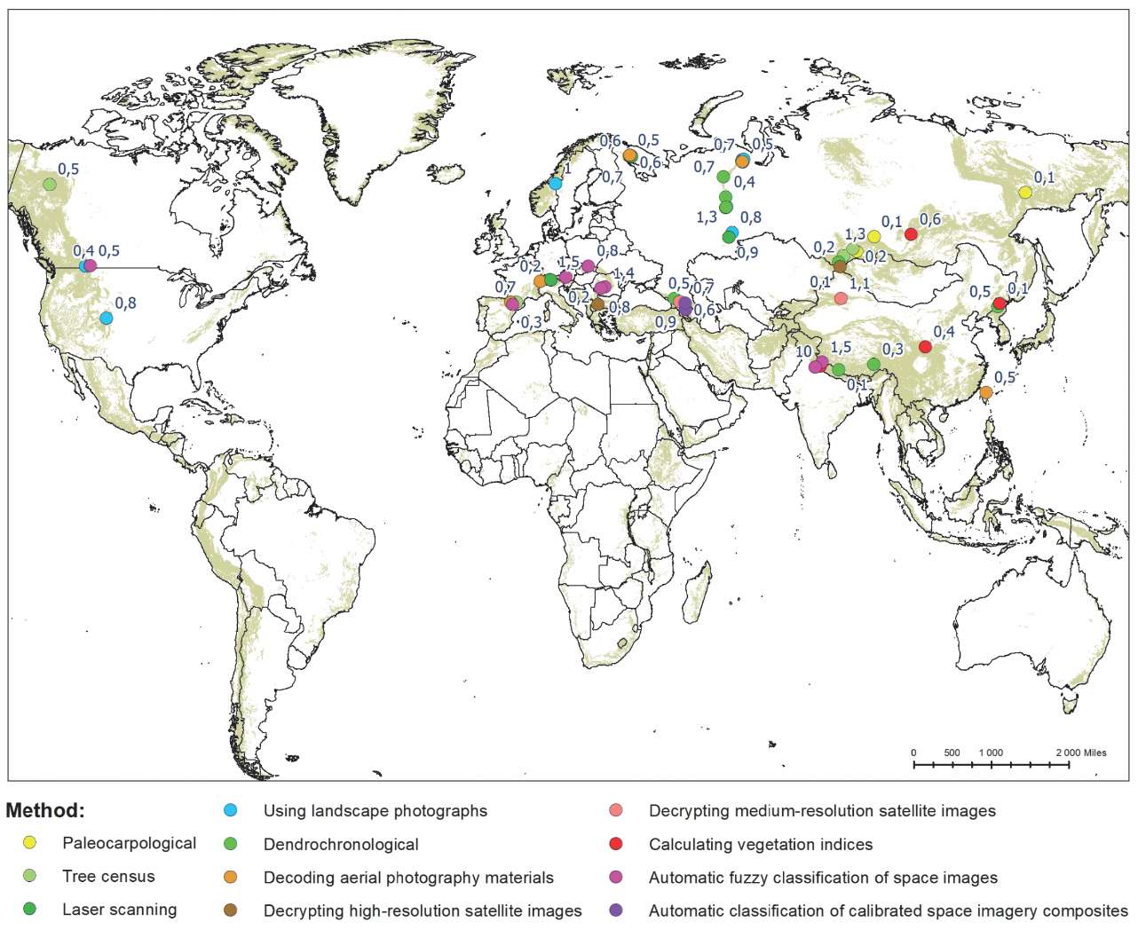
Fig. 1. Places of study of the alpine treeline; values near a point indicate the average speed of the dynamics (meters per year), the color of the point corresponds to the type of research method
It would seem that the processing of remote sensing data with modern methods of geostatistical analysis allows obtaining data on the localization and transformation of the ATL at any spatial level, including the regional one. All current ways of classifying space images rely on local samples for training. These samples might not fully capture the true complexity of the landscape and the specific patterns found in the ATL ecotone. It has been assumed that an accurate assessment of the forest boundary dynamics requires synthetic methods using complex models that consider differentiation at the landscape site scale (facies, elemental landscapes) and that are based on a preliminary understanding of the features of the landscape pattern, so this makes its further interpolation possible at the landscape scales or larger natural units, i.e., physical–geographical regions and countries (Grabherr et al. 2000).
The concept of the upper forest boundary has undergone significant over time. The idea of the boundary as a ‘line’ is recognized as an unacceptable simplification by researchers of various fields (geobotanists, ecologists, and last but not least, landscape science specialists). It may be considered that the ATL is a kind of strip, a transition between ‘forest’ and ‘non-forest’ zones, which varies in width and configuration; its complexity is largely determined by a set of landscape-forming conditions. In this work, the ATL is understood as an ecotone that records the transition from the closed forest canopy to the treeless space in a gradient of deteriorating heat and moisture exchange conditions. The variety of ecotones depends on the types of forests. These can include groups of coniferous or deciduous trees, elfin woodland, or mixed morphological forms of woody vegetation from different species. On the other hand, these can be the types of open spaces, as the latter can be represented by shrub thickets (e.g. rhododendrons), alpine meadows, and mountain tundra with moss and shrub ground covers.
At the present time, the conceptual framework for studying the ATL is preconditioned by the parameters that characterize the state and dynamics of the ATL, the development of models that explain the driving factors of ATL dynamics, the assessment of the stability of dynamics (short-term dynamics or trends), the representativeness of the identified patterns, and the possibility of their application in other regions.
We searched ISI Web of Science, Scopus Preview, Springer Nature, ResearchGate, Refseek, BioOne Digital Library, Bioline International and eLIBRARY databases for scientific articles published since 1995 using the following set of keywords in Russian (“верхняя граница леса” OR “граница леса” OR “верхние границы леса” OR “верхняя граница древесной растительности” OR “динамика границ поясов” OR “экотон верхней границы древесной растительности”) and English (“Alpine tree line” OR “Alpine treeline ecotone” OR “Treeline, Tree line, Timberline, Treeline ecotone” OR “Tree line advance” OR “Tree line dynamics” OR “Treeline ecotone dynamics” OR “Tree line change rate” OR “Dynamics of borders of belts” OR “Tree stand dynamics and Upper tree-line”).
Simultaneously, we selected combinations of terms found in the headings of articles, annotations and keywords that appealed to techniques using remote sensing data and their processing algorithms: “космические снимки” OR “повторные ландшафтные фотографии” OR “снимки сверхвысокого разрешения” OR “лазерное сканирование” OR “дендрохронологический анализ” OR “remote sensing” (Image classification, Change detection, Repeat photography, Dendroecology, Convolutional neural network, Landsat and LiDAR).
Also, we looked at full-scale literature reviews, including those by F.K. Holtmeier and G. Broll (2019) and P.J. Morley and others (2018), as well as the reference lists from the articles we studied. We excluded articles that looked at the physiological and developmental processes of the ATL but did not examine the changes in the ecotone from the dataset. Due to the disproportionate quantitative predominance of articles on dendrochronological topics, general publications devoted to the main mountain regions of the world were selected from the total pool. If one author had a number of studies published, the article that most reflected the applied methodology and results of the study was taken for the analysis.
The search yielded 591 articles, 55 of which were finally considered after omitting the publications that did not meet the selection criteria and duplicates. The sorting was performed according to the ROSES flow chart for systematic reviews (Haddaway et al. 2017). The articles examined for this analysis discussed various methods used to study the changes in the ATL in the major mountain ranges of Eurasia and North America.
As a result, the final list included only those articles that contained descriptions of methods for studying the ATL and included the following parameters: area of the territory under study, height and localization of the ATL,
The interpretation and comparison of the obtained data also considered the geographical features of the study regions, primarily the role of the anthropogenic factor (see Supplementary material). The data collected in this review have been analyzed using R1. The map of the spatial distribution of cases was created using QGIS2, where the mountain systems (yellow) are presented according to the model of the Global Mountain Biodiversity Assessment (GMBA) (Snethlage et al. 2022).
Counting tree volume and determining the age of trees using drilling represent one of the oldest methods for studying the ATL in the mountains; this is an integral part of forest taxation. The technique consists of laying out test zones at model areas, where taxation parameters are measured for each tree, and the core is extracted with a Pressler drill borer at a height of up to 30 cm from the ground surface. Specialized semi-automatic measuring systems, such as LINTAB and TSAP, are used to measure the width of the growth rings with high accuracy (up to 0.01 mm) and cross-date samples. The COFECHA (DPL) program then performs additional dating control. Individual cross-matched chronologies are standardized using a negative exponential or linear regression. The ARSTAN program is used to standardize and calculate general chronologies by averaging individual data series.
This technique has been widely applied in vast territories. Some example ATL studies were conducted in the Khibiny Mountains of the Kola Peninsula (Konstantinov and Volkov 2022), the Caucasus (Dyakonov and Bochkarev 2012), the Altai Mountains (Bocharov 2011), the Western Sayan Mountains (Istomov 2005), the Tuva Republic (Russia; Kolunchukova and Reznikov 2020), the Nepalese Himalayas (Shrestha et al. 2015), the Tibetan Plateau (Liang et al. 2011), the eastern and western mountain systems of China (Du et al. 2018; Wang et al. 2022), the western part of the Mackenzie Mountains (Mamet and Kershaw 2012), the Central Alps (Frei et al. 2023) and the Pyrenees (Batllori et al. 2010).
Recent tree census studies have begun to use high-tech tools, such as laser scanning methods. A review of the application of this method can be found in a number of papers, particularly studies performed at the Southern Urals (Vorobyeva et al. 2022), the Swiss Alps (Coops et al. 2013) and the Khibiny Mountains (Nisametdinow et al. 2021). Processed LiDAR data obtained from airborne or ground platforms makes it possible to remotely map tree trunks and shrubs in the transition zone with high accuracy and determine their characteristics, which allows one to expand the research area significantly.
Paleocarpological studies of peat deposits provide the deepest chronological section (up to 4,000 years) of forest boundary dynamics. The technique involves taking kerns in Pleistocene deposits and obtaining organic fractions from them. Carpological remains (seeds, fruits, and megaspores) are identified by referring to collections of fossil carpoids. The results are analyzed by the method of carpological diagrams (the number of taxa remains in a sample of 100 cm3) using specialized programs, such as TILIA. As a result of the reconstruction of coastal and marsh vegetation, based on the analysis of coenotic groups of species, a model of changes in the altitudinal ranges is obtained.
Due to the limited distribution of peat deposits in the ATL and approximate estimates of the dynamics, this method is rarely used in the mountains. Currently, the known studied research areas are only the mountainous territories in Russia: the Sayan Mountains, mountains in the Tuva Republic, and Eastern Siberia (Koshkarov et al. 2019; Lytkin 2019; Murzakmatov et al. 2014).
The method of comparing the historical and modern landscape photographs taken from the same points has proven itself in various mountainous regions (Webb, Boyer 2010). In addition to the visual processing of landscape photographs, the algorithm includes the bookmarking of height profiles, collecting dendrochronological samples, and considering growth tables of forest stands to obtain quantitative characteristics of the latter based on landscape photographs. Usually, a transformed grid is built for the analysis of photographs, and each grid cell is assigned an attribute of vegetation condition. Covariance analysis methods are used to process the obtained matrices.
The technique has long been used in Russia for the Polar, Subpolar, and Southern Urals, where the images first taken in the 1960s were used for comparison (Grigor’ev et al. 2013; Nikolin et al. 2015; Shiyatov 2009; Shiyatov, Mazepa, Moiseev 2001; Shiyatov and Terentyev 2005). In Canada, the photographs taken in 1914 were compared with LiDAR data and repeated photographs from the Mountain Legacy Project in the West Castle Watershed (Alberta) (McCaffrey and Hopkinson 2020). In the USA, a large set of photographs taken over a period of 148 years was analyzed (Peterson et al. 2022). A similar method for the visual determination of the ATL was used in Scandinavia (Kullman and Öberg 2009). Changes in tree height in southern Sweden were quantified for the period 1915–2007 and for two time periods of 1915–1975 and 1975–2007, separately. The algorithm used repeated trips to monitoring sites (altitude belt transects) and measurements of treeline position (in meters above sea level) during the three specific periods.
The method is quite simple, but the authors note its shortcomings, which are the inaccuracies arising during interpretations in the laboratory and the locality of the data obtained, which does not allow the wide extrapolation of the research results.
Dendrochronological analysis is still the most widely used method for studying the ATL. It involves measuring the width of the wood rings from the scanned images of tree trunk cores taken from the study area and their subsequent analysis using statistical processing programs designed especially for dendrochronological series, such as the International Dendrochronological Library, or general statistical software, such as R Core Team. The results of the analysis make it possible to confirm the correlation of tree growth changes with astrophysical (sun position, solar activity), climatic (average monthly positive air temperatures) and geomorphometric (slope gradient and aspect) parameters; the presence of permafrost; the peat layer thickness in soils; the frequency of avalanches; land use; and other factors. Dendrological data allow one to estimate the trends of temporal changes in growth for the region under study and allocate the main parameters of the system’s response to climatic fluctuations. Dendrochronological analysis methods are often used together with ground mapping techniques. The limitations of this method are the choice and use of only adult trees for coring without studying other components of the ATL and the locality, the limitation and the complexity of the interpolation of results.
The most systematic and long-term studies using dendrochronological methods were conducted in the Northern and Subpolar Urals (Devi et al. 2018; Dyakonov and Bochkarev 2012; Galaco 2002; Kapralov 2007; Mazepa and Shiyatov 2015; Moiseev and Nagimov 2010; Moiseev et al. 2008). Other important research in mountain regions was done in the Elbrus area of the Caucasus (Dyakonov and Bochkarev 2012), the Tibetan Plateau (Liang et al. 2011), the Changbai Mountains (Du et al. 2018) and the Nepalese Himalayas (Shrestha et al. 2015).
The trends in ATL dynamics were studied comprehensively over the past century (1901–2004) using tree-ring width data from 13 regions representing most of the key mountain landscapes of Eurasia and America (Camarero et al. 2021). A general increase in the treeline altitude was noted during the 20th century, with the trend becoming most pronounced since the 1980s. A positive relationship between tree growth rates and growing season temperatures was confirmed. The highest growth rates, against the background of pronounced warming, were recorded in the Pyrenees; declines in growth rates were found in some areas in the Rocky Mountains and Scandinavian Mountains. For mountain rainforests of the Southern Hemisphere, significant positive growth trends turned out to be relatively independent of the relatively weakly changed temperature background (in both winter and summer seasons). It was suggested that in the 21st century, tree growth and the rise of the ATL will cease to depend directly on the temperature factor in all mountainous regions of the world.
The method of decoding multi-temporal aerial photography of the Earth's surface makes it possible to obtain spatial data on the changes in the upper forest boundary. The algorithm includes procedures for bringing historical aerial images into a single projection, combined with modern satellite images and vector maps of a similar scale. This results in fixing the contrastingly visible forest boundary and comparing the localization using geostatistical tools. The method was used in a study of Taiwan's mountain forests, where a clearly visible forest boundary was drawn using aerial photographs from 1963, 1975, and 2001, and then the contours were compared (Greenwood et al. 2014). At the Polar Urals, aerial photography materials from 1962 and 1964 were used (Mikhailovich 2016). The upward shift of the sparse forest boundary here was assessed on the basis of aerial photography using a digital elevation model in the ArcGIS program (Nizametdinov et al. 2022).
A study on the Catalan Pyrenees used more than 200 pairs of aerial photographs taken 50 years apart, in 1956 and 2006 (Ameztegui et al. 2016). Neural networks were used to analyze aerial photographs in the Swiss Alps, which helped estimate changes in the ATL over 30 years, using black and white aerial photographs taken in 1980 and 2010 (Wang et al. 2022). In this case, a convolutional neural network model was first created based on three classes of objects calculated from airborne laser scanning data, considering black and white aerial photographs from 2010; then, the model was trained on the samples of historical black and white aerial photographs from 1980.
To compare the ATL of different periods, forest boundaries taken from the military topographic maps are sometimes used. In Russia, the latter were developed on the basis of decoding aerial photographs. For example, topographic maps (scale 1:50,000) linked to IRS LISS/PAN space images were used in the study of the Khibiny Mountains (Mikheeva 2010).
The method of ATL mapping based on an expert interpretation of space images is similar to the aerial photography method. This method usually uses high-resolution photography (1–5 m per pixel) comparable to the scale of the considered aerial photographs (typically 1:10,000).
For example, in a study of forest boundary changes in the Sangun River watershed in the Tianshan Mountains (Xinjiang, China), a 2006 QuickBird image was compared with aerial photographs from 1962 and 1981. Segmentation methods using an object-oriented image classification algorithm were applied (Luo and Dai 2013).
In the Khibiny Mountains, the results of interpreting high-resolution space images from 2001 and archival aerial photographs from 1958 were compared based on the classification of landscapes in ERDAS Imagine using the maximum similarity algorithm (Mathisen et al. 2014). Hexagon images obtained in 1976 were used for similar purposes in the study of the Belasitsa Mountains along the border between the Republic of Bulgaria and the Republic of Macedonia (Groen et al. 2012).
All studies using aerial photographs and high-resolution satellite images are local in nature (from 1 to 10 km²), which is due to the labor-intensive nature of manual decryption, limited access to relevant archives, and significantly different quality of historical sources. In addition, the use of modern aerial photography for regional analysis is always difficult due to objective circumstances. Collecting a full set of data is not only associated with large expenditures of time and money but also requires an ‘ideal weather’ (a certain number of clear days). Overall, the inconsistent data from images taken at different times and the varied geographic coverage make it difficult to apply the research findings to larger regions or countries.
The method of interpreting multi-temporal images of the Landsat and Sentinel satellite series (resolution of 10–30 m/pixel) is used to obtain spatial estimates of the dynamics of mountain forests, when the latter are supported by the available standards of the survey sites (collected during field studies). The delimitation of mountain forests is manually carried out visually, via semi-automatic algorithms, such as maximum similarity in ERDAS Imagine (Kravtsova and Loshkareva 2010); or by means of the GRASS GIS (Zhuravleva, Karanin 2017). Object-oriented classification algorithms using the Definiens eCognition 25 software were also used (Luo and Dai 2013). For example, when studying the dynamics of mountain forests in the Caucasus, the supervised classification method in the ArcGIS program was used to process multi-temporal images of Landsat-5 taken in 1988 and Landsat-7 in 2017 (Alekseeva 2021). In the Tien Shan Mountains, an analysis was carried out via the maximum likelihood method using GRASS GIS tools (Zhang et al. 2021).
Calculating vegetation indices is the most common method of the automatic analysis of multi-temporal medium-resolution images. It allows the normalization of the images taken by different equipment and thus eliminates interpretation errors. In these studies, the normalized difference vegetation index (NDVI) is calculated by comparing the infrared (near infrared) and visible (red) reflected signal, which can characterize vegetation types and their condition.
For example, Landsat images of the Baikal Ridge in 1975 and 2010 were compared. Changes in the vegetation cover here were determined using the NDVI index calculated from satellite images (Vladimirov 2014). Images from Landsat 5 (1987) and Landsat 8 (2020) of the Taibai Mountain in China converted into vegetation indices were processed using ENVI software module to create vegetation indices with regression analysis (Wang et al. 2022). In a similar study of ATL dynamics at the Changbai Mountains in northeastern China, Landsat images from 1977–1999 were used to obtain the ratio of the calculated normalized vegetation index of birch and coniferous forests at the upper boundary of their distribution (Zhang et al. 2009). In the Indian Himalaya region, IRS-P6, LISS-III, and Landsat MSS images were used from 1972 to 2006, so threshold values of forest edge NDVI were determined; finally, the rate and magnitude of change were calculated using geostatistical analysis methods (Singh et al. 2012).
Discrete classifications are useful for ATL studies, especially for studying the relationships between the mosaicity of the edge of high-mountain forests and the processes predetermining such mosaicity, as it becomes possible to correlate the characteristics of vegetation types with the field data and published descriptions. However, these methods work only where there is a correlation between the spectral characteristics and observed ground features of objects. No quantitative assessment of the degree of variation in the structures of the ATLs – reflected in the spectral characteristics of the objects that comprise them – has been made so far.
The most recent methods process medium-resolution images using a variety of automatic space image classifications. These methods are mainly applied to the images obtained by Landsat series space satellites. The Landsat archive is the most complete archive of medium-resolution space images, with 80-m/pixel images available since 1973 and 30-m/pixel images available since 1982. The duration and precise spatial referencing of Landsat archive data allow for a qualitative assessment of the changes in landscape objects at the macroregion level without additional spatial and brightness corrections. This makes it the best candidate for automatic image classification methods.
In a study on the ATL in the Himalayas, Landsat 5/8 satellite data from 1989–2015 were used to create NDVI and normalized difference snow index (NDSI) raster for a further application of the classification process by a neural network–based algorithm, such as a decision tree (Sushma et al. 2010; Zhang et al. 2021).
Landsat ETM images from 2002 and OLI images from 2015 were analyzed for the Jizera Mountains, the Southern Carpathians, Romania (Mihai et al. 2017). Thematic classification was done using the maximum likelihood algorithm, which is based on calculating the Gaussian probability around each training set of pixels. The training set was based on the forest stand data from INCDS Bucharest (National Institute for Forestry Research and Development).
Landsat satellite images for the periods of 1971–1980, 1981–1990, 1991–2000 and 2001–2014 were analyzed for a large-scale study of the national parks evenly distributed across the dominant European mountain ranges, such as the Pyrenees, the Alps, and the Carpathians (Dinca et al. 2017). Changes in forest boundaries were measured using the post-classification comparison algorithm.
Multi-temporal Landsat TM data (1988–1990) were used to map alpine forests in Montana (Allen and Walsh 1996). Cluster analysis based on the relationship with forest reflectance was applied to create models for each temporal boundary in the compared images. A similar study was conducted in the western Himalayas, where Landsat MSS and TM images over a 30-year period from 1980 to 2010 were used (Bharti et al. 2012). For supervised classification, training signatures of six different classes were specified based on in situ data collected during field surveys. Signatures were assessed for a possible separation of individual classes using the ERDAS transformed divergence method.
Fuzzy classification is an attractive alternative to expert (‘manual’) ecotone mapping, where there are no clear boundaries among vegetation classes. Fuzzy classification pre-assigns a score for individual pixels based on the so-called fuzzy membership of the pixel to a finite class. The fuzzy membership itself may be set in different ways in modern GIS tools, which gives the researcher much flexibility to test the algorithm and find an optimal solution. However, in most studies, the use of such fuzzy logic algorithms is limited to the territory of a single Landsat image because normalizing a mosaic of images with different times and angle characteristics is quite a complex process. In addition, the lack of accompanying field data for each image in a series results in the accumulation of interpretation errors when analyzing images of different periods. When using only two images taken within a significant period, the classification error in each image may lead to an incorrect interpretation of changes that do not reflect the real pattern. The use of a continuous multi-temporal series of space images may become a solution to this issue.
There are scarce publications aimed at solving the issues of normalizing the mosaics of satellite images and of developing continuous time series. These methods are used to create continuously calibrated composites from the stacks of Landsat space scenes to fill in the gaps associated with cloudiness or haze and develop the sets of phenological and statistical metrics, which can be analyzed by the neural network–based models (Potapov et al. 2020).
A large-scale study of landscape dynamics in the Caucasus (Buchner et al. 2020) used composites of 12651 Landsat images from 1985 to 2016 (all available images with less than 70% cloud cover). The FORCE mask algorithm was used to fill in the gaps. Based on the composites, phenological metrics were calculated using the spline analysis of the time series algorithm associated with climate variability, such as the beginning of the vegetation growth season, its peak, and its end. Correlations of phenological metrics with the algorithm-selected (based on neural networks) landscape/land cover classes (LandCover/LandUse) were established; these classes comprised, but were not limited to, coniferous forests, mixed forests, deciduous forests, barren lands, pastures, croplands, built-up lands, wetlands, water, snow, and ice. To obtain training samples, the corresponding objects (polygons) verified in the field were digitized on high-resolution images.
When studying the dynamics of landscapes in the North Caucasus in our previous studies, processed Landsat analysis ready data (ARD) were analyzed as 16-day composite data normalized by reflectivity (for the visible, near and shortwave-infrared bands of the channels) and by data quality (Purekhovsky, Gunya, Kolbovsky 2022). Areas covered by clouds and haze were corrected based on cloud-free images using a specialized gap-filling method. Annual 16-day GLAD ARD time series were transformed into a set of ranked statistical data (phenological indicators), which made it possible to apply multi-temporal classification and regression models. For each ranking, a set of indicators was calculated, including selected ranks, inter-rank averages, and amplitudes. In addition, a set of indicators reflecting seasonal changes associated with the main stages of vegetation was calculated based on the NDVI index. Phenological metrics were supplemented with geomorphometric indicators (absolute height and slope gradient). The analysis used an algorithm based on neural networks (such as a decision tree); training took place on an array of test objects obtained by analyzing high-resolution space photography and in-kind data.
The methods for studying the ATL may be divided into several groups based on methodology (e.g. in situ, remote and their combinations), spatial and temporal scales, parameters measured, and efficiency and limitations of application (Table 1).
Table. 1. Comparative characteristics of ATL study methods
Methods | Main measured parameters | Spatial size | Time period | Limitations and drawbacks |
Paleocarpological methods | Tree composition | Key areas N × 10 km² | Thousands of years | Rare occurrence of peat deposits in highlands |
Tree census | Change in the number of trees and timber volume | Key areas N × 100 km², less often N × 1000 km² | For several hundred years | Locality, difficulty in ensuring representativeness and extrapolation to large areas |
Laser scanning methods | Spatial structure of tree cover of ATL on a large scale and its transformation | N × 1000 km² | For decades | Labor-intensive and costly, difficult to ensure representativeness and extrapolation |
Method of using landscape photographs | Qualitative (expert) assessment of the trend of change in the boundaries of the ATL on a large size | N × 100 m² - N × 1000 m² | Decades, rarely hundreds of years | Limited number of places provided by historic landscape photographs, difficulty in applying accurate algorithms to analyze photographs |
Dendrochronological method | Estimation of wood growth trend based on tree ring width measurements | N × 100 m² - N × 1000 m² | For several hundred years | Focus on mature trees, without surveying other components of ATL; Localized, difficult to ensure extrapolation to other areas |
Method of decoding aerial photography materials | Spatial structure and boundary of the ATL ecotone on a large scale | N × 10 km², less often N × 100 km² | For decades | Limited number of places with availability of historical maps, the difficulty of selecting multitemporal imagery of equal resolution, necessity for ground verification |
Method for decrypting high-resolution satellite images | Spatial boundary of the ATL ecotone and its changes on a large scale | N × 100 km² | For decades | Limited number of locations with availability of multi-temporal images of equal resolution |
Method for decrypting medium-resolution satellite images | Medium-scale localization and configuration of ATLs based on the identification of vegetation cover types | N × 100 km² | For decades | The problem of labor-intensive manual processing of large coverage, inaccuracy of the result by automatic classification method without training |
Method of calculating vegetation indices | Medium-scale localization and configuration of ATLs based on the identification of vegetation cover types | N × 1000 km² | For decades | The problem of identifying the mature forest boundary, without investigating other components of the ATL, the need for ground verification |
Method of automatic fuzzy classification of space images | Localization of ATL and its configurations on a medium scale | N × 10,000 km² | For decades | Error of automatic processing of images of different quality and partially cloud-covered images, necessity of ground verification |
Method for automatic classification of calibrated space imagery composites | Localization and configuration of ATLs: dimensionality parameters (area, width) of the encompassing ecotone | N × 100,000 km² | For decades | Large volumes of data analyzed, complexity of simultaneous processing of data from different natural zones, the need for training |
The present review allows for tracking the changes and evolution of methods for studying the ATL. The primary methods were the modified forest inventory practices; therefore, they were based exclusively on the data collected in the field. Emphasis was put on the tree age data, which served as a basis for obtaining a final model of standing growth and development within the ATL ecotone. The development of this approach was limited by the possibilities provided by the field taxation description of stand characteristics; subsequently, these possibilities were significantly expanded by the use of dendrochronological analysis. The use of LiDAR imaging technology made it possible to record the stand structure with much greater accuracy. However, when using this method, there was an acute lack of spatial information for approximating and extrapolating data to large areas. These limitations were overcome in part through the use of aerial photography and historical photographs of the mountains.
Nevertheless, a breakthrough in ATL study methods is associated with the introduction of remote sensing data into scientific practice, primarily remote sensing materials from repeated surveys. First, they were tested for small key areas and then in ever-expanding territories. At the same time, the transition from the local to the regional and global levels was accompanied by an exponentially increasing labor intensity of interpretation, which required procedure automation and an almost complete rejection of expert (manual) methods of analysis. The development of methods for semi-automatic (controlled by an expert) and automatic (uncontrolled) processing of space images resulted in promoting various classification (‘segmentation’) algorithms for vegetation cover and land-use types, with subsequent comparisons among the boundaries of the identified vegetation types. The introduction of appropriate tools into modern GIS software provided researchers with the ability to process data for large areas and even entire mountain systems. At first, these methods were relatively simple (e.g. calculating vegetation indices), but with training and the use of machine learning algorithms based on neural networks, classification methods began to be applied as GIS analysis technologies were being developed (Fig. 2).
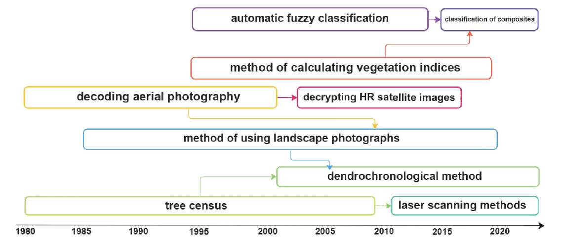
Fig. 2. Development of methods for ATL studying
The effectiveness of methods for studying the dynamics and transformation of the ATL is predetermined mainly by the ratio of two main parameters: (1) the size (area) of the studied territory and (2) the time range of the recorded changes. The study area predetermines the data volume to analyze, which, in turn, affects the accuracy largely, bringing some limitations at local and regional scales and thus influencing model correctness. The time depth makes it possible to separate the average long-term trends from random fluctuations of the ATL.
Field methods, such as tree census and dendrochronological analysis, allow for the building of models with a uniquely significant time interval (from 30 to 800 years). However, they still cover extremely small areas of model plots (less than 0.5 km²). Aerial photography and high-resolution space imagery make it possible to record the ATL changes over the past 20–60 years. However, the analyzed area may cover dozens of thousands of square kilometers, which is commensurate with the size of a physical–geographical region. The methods for the automatic processing of medium-resolution space photography with a relatively low time depth (the last 20–40 years) make it possible to study the areas of hundreds of thousands of square kilometers, which is equal to the size of an entire mountainous country.
The obtained correlation of the area of the study territory with the time coverage was 0.45 (Fig. 3), demonstrating a clearly traceable trend towards an increase in the area of the study territory, which meets the request for an analysis of the dynamics of the ATL on the scale of large regions, physical–geographical territories, and administrative states.
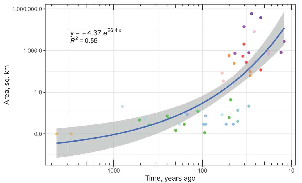
Fig. 3. Correlation of area and time parameters of the ATL dynamics methods. The colors are indicated by different methods. The color designations are shown in Fig. 1
Analysis of accumulated experience in the application of various approaches and methods for studying the localization and average annual dynamics of the ATL allows for coming up with a list of urgent issues and needs. The ATL, being a relatively narrow ecotone, is, nevertheless, widely distributed in various mountain systems at the global level. As a result, it is characterized by a significant variety of location conditions. Therefore, searching for or applying an ‘ideal’ method for ATL studying is unreal.
The most common field methods (tree census, dendrological analysis and paleocarpological studies) require a large volume of fieldwork, which is especially difficult in rugged mountainous terrain. This predetermines the extremely limited (practically ‘point-scale’) information obtained, which is intended to be applied to analyze the trends in large regions. Landscape photographs aid in partially solving this issue, but their use is very localized and limited by the lack of vast archives of such photographs.
The methods based on the processing of remote sensing data may serve as a solution to the issue of achieving broadly applied and reliable extrapolation. These methods help to develop spatial models of forest boundary changes at the administrative-state, subcontinental, and global scales. However, these innovative approaches also have many limitations. High-resolution images (similar to aerial photography in scale and accuracy), which allow visual identification of individual tree crowns, are usually limited to the boundaries of a single scene (an area of up to several hundred square kilometers). This is associated with their high cost and the large amount of manual labor required for processing. Medium-resolution images, in which the pixel resolution is greater than the size of the tree crown, require complex classification during analysis that identifies transitional classes of vegetation and corresponds to a complex mosaic of the distribution of species and the morphotypes of tree and shrub vegetation (i.e. crooked forests and dwarf trees) at the boundary of their altitudinal distribution.
Nowadays, the data obtained by the Landsat satellite system (30 m per pixel) is the most effective in analyzing vast territories due to their standard nature and the accuracy of the reference determined by the stability of satellite orientation. Compared to the Landsat archives, Sentinel 2 images, available since 2016, have an improved resolution (10 m per pixel). However, these satellites can operate for less than 10 years, which does not provide sufficient time depth to draw any conclusions about the average long-term dynamics of the ATL using this method. Combining the data from these two series would allow for operating with a depth of up to 50 years, alongside maintaining the image resolution, but this is possible only when using the integral composites.
The contradiction between the accuracy of measurements and the area of the studied territories is a classic problem that characterizes the applicability of remote sensing data. The correction of the results of ATL modeling in mountainous conditions encounters poor accessibility to highlands for field verification methods. Many studies are based on random, point-distributed modern or historical data and surface images covering local model areas. Such studies consider the observations at key sites only and are thus required to be representative when extrapolated to larger territories. To solve the issue of data extrapolation, it is necessary to develop spatial models of ATL changes based on remote sensing data.
Most researchers find a compromise by processing available medium-resolution images using segmentation methods with an excessive simplification of forest classes when studying the ATL. However, at the altitudinal limit of forest distribution, the ecotone transformation mostly refers to the tree growth and the rooting of the species presented rather than to changes in community biodiversity and composition. Therefore, in the classifications obtained by analyzing the remote sensing data, it is necessary to identify young trees first, as both their number and spatial distribution affect the direction and rate of ATL dynamics. Simple classifications alone cannot accomplish this without training.
Combining methods based on automatic nonlinear classification of medium-resolution space images with training on field and office research data obtained by other techniques may become a solution to the issue stated above. Transformation (or conversion) tables developed in regard to dendrochronological, counting (census) and other field methods of collecting and processing materials could serve as a basis for creating the arrays of objects and models for training algorithms built with neural networks. The use of detailed laser scanning data to train a neural network to interpret Landsat composites is a worthy example of such an approach (Potapov et al. 2021).
Most methods aim to delineate the ecotone boundaries, tracking boundary shifts among landscape–altitude belts (forest, alpine meadow, and nival). However, only some of them allow for the identification of the qualitative changes within the ecotone itself in association with its horizontal and vertical structures and are not necessarily accompanied by a shift in the ATL. Assessing the changes in terms of attributing them to cyclical or unidirectional average long-term trends is another important issue. Short-term and/or local observations, which have revealed the transformation of the ATL, do not allow one to establish the stability and direction of changes reliably. Finally, both the interpretation of ATL changes and the search for independent variables in the corresponding models often suffer from an overestimation of climatic fluctuations as leading factors, while other important factors, primarily human activity, remain undisclosed or are deliberately ignored. The latter are based on the idea of a pristine environment in mountain forests, which is not true in a number of cases. As a result, the methods currently used to study the altitudinal–zonal (landscape) forest boundary are mostly effective only at the local or, at best, regional scales; when attempting to extrapolate, they often lead to incorrect conclusions.
A critical analysis of the experience accumulated to date in studying the localization and average long-term dynamics of the ATL indicates the need to create synthetic solutions. They must be based on both (1) using the metrics of holistic composites of medium-resolution space imagery and (2) considering large arrays of field-obtained data on the position (for training machine learning algorithms), internal spatial organization and characteristics of forest communities in mountainous countries around the world.
1. R Core Team (2023). R: A Language and Environment for Statistical Computing. R Foundation for Statistical Computing. Vienna, Austria. URL: https://www.R-project.org.
2. QGIS Development Team (2019). QGIS Geographic Information System. Open-Source Geospatial
1. Alekseeva N. N., Gunya A.N., Cherkasova A.A. (2021). Land cover dynamics during recent 30 years (case study of the "Alanya" National park, the Northern Caucasus). Lomonosov Geography Journal, (2), 92–102, (in Russian with English summary).
2. Allen T.R. and Walsh S.J. (1996). Spatial and compositional pattern of alpine treeline, Glacier National Park, Montana. Photogrammetric Engineering and Remote Sensing, 62(11), 1261–1268.
3. Ameztegui A., Coll L., Brotons L. and Ninot J.M. (2016). Land-use legacies rather than climate change are driving the recent upward shift of the mountain tree line in the Pyrenees. Global Ecology and Biogeography, 25(3), 263–273, DOI: 10.1111/geb.12407
4. Batllori E., Camarero J.J. and Gutiérrez E. (2010). Current regeneration patterns at the tree line in the Pyrenees indicate similar recruitment processes irrespective of the past disturbance regime. Journal of Biogeography, 37(10), 1938–1950, DOI: 10.1111/j.1365-2699.2010.02348.x
5. Bharti R.R., Adhikari B.S. and Rawat G.S. (2012). Assessing vegetation changes in timberline ecotone of Nanda Devi National Park, Uttarakhand. International Journal of Applied Earth Observation and Geoinformation, 18(1), 472–479, DOI: 10.1016/j.jag.2011.09.018
6. Bocharov A.Yu. (2011). Structure and dynamics of high-mountain forests of the North Chuysky Ridge (Altai Mountains) under climate change conditions. Bulletin of Tomsk State University, (352), 203–206, (in Russian with English summary).
7. Buchner J., Yin H., Frantz D., Kuemmerle T., Askerov E., Bakuradze T., Bleyhl B., Elizbarashvili N., Komarova A., Lewińska K.E., Rizayeva A., Sayadyan H., Tan B., Tepanosyan G., Zazanashvili N. and Radeloff V.C. (2020). Land-cover change in the Caucasus Mountains since 1987 based on the topographic correction of multi-temporal Landsat composites. Remote Sensing of Environment, 248(September 2019), 111967, DOI: 10.1016/j.rse.2020.111967
8. Calvin K., Dasgupta D., Krinner G., Mukherji A., Thorne P.W., Trisos C., Romero J., Aldunce P., Barrett K., Blanco G., Cheung W.W.L., Connors S., Denton F., Diongue-Niang A., Dodman D., Garschagen M., Geden O., Hayward B., Jones C., … Ha M. (2023). IPCC, 2023: Climate Change 2023: Synthesis Report. Contribution of Working Groups I, II and III to the Sixth Assessment Report of the Intergovernmental Panel on Climate Change [Core Writing Team, H. Lee and J. Romero (eds.)]. IPCC, Geneva, Switzerland. , P. Arias, M. Bustamante, I. Elgizouli, G. Flato, M. Howden, C. Méndez-Vallejo, J. J. Pereira, R. Pichs-Madruga, S. K. Rose, Y. Saheb, R. Sánchez Rodríguez, D. Ürge-Vorsatz, C. Xiao, N. Yassaa, J. Romero, J. Kim, E. F. Haites, Y. Jung, R. Stavins, … C. Péan eds. DOI: 10.59327/IPCC/AR6-9789291691647
9. Camarero J.J., Gazol A., Sánchez-Salguero R., Fajardo A., McIntire E.J.B., Gutiérrez E., Batllori E., Boudreau S., Carrer M., Diez J., Dufour-Tremblay G., Gaire N.P., Hofgaard A., Jomelli V., Kirdyanov A. V., Lévesque E., Liang E., Linares J.C., Mathisen I.E., … Wilmking M. (2021). Global fading of the temperature–growth coupling at alpine and polar treelines. Global Change Biology, 27(9), 1879–1889, DOI: 10.1111/gcb.15530
10. Chen I.C., Hill J.K., Ohlemüller R., Roy D.B. and Thomas C.D. (2011). Rapid range shifts of species associated with high levels of climate warming. Science, 333(6045), 1024–1026, DOI: 10.1126/SCIENCE.1206432/SUPPL_FILE/CHEN.SOM.PDF
11. Coops N.C., Morsdorf F., Schaepman M.E. and Zimmermann N.E. (2013). Characterization of an alpine tree line using airborne LiDAR data and physiological modeling. Global Change Biology, 19(12), 3808–3821, DOI: 10.1111/gcb.12319
12. Däniker A. (1923). Biologische Studien über Wald- und Baumgrenze, insbesondere über die klimatischen Ursachenund deren Zusammenhänge. Vierteljahresschr. Naturfr. Ges. Zürich, 63, 1–102.
13. Devi N.M., Kukarskih V.V., Galimova A.A., Bubnov M.O. and Zykov S.V. (2018). Modern Dynamics of High-Mountain Forests in the Northern Urals: Major Trends. Journal of Siberian Federal University. Biology, 11(3), 248–259, DOI: 10.17516/1997-1389-0069
14. Devos C.C., Ohlson M., Næsset E. and Bollandsås O.M. (2022). Soil carbon stocks in forest-tundra ecotones along a 500 km latitudinal gradient in northern Norway. Scientific Reports, 12(1), 13358, DOI: 10.1038/s41598-022-17409-3
15. Dinca L., Nita M., Hofgaard A., Alados C., Broll G., Borz S., Wertz B. and Monteiro A. (2017). Forests dynamics in the montane–alpine boundary: a comparative study using satellite imagery and climate data. Climate Research, 73(1–2), 97–110. DOI: 10.3354/cr01452
16. Du H., Liu J., Li M., Büntgen U., Yang Y., Wang L., Wu Z. and He H.S. (2018). Warming-induced upward migration of the alpine treeline in the Changbai Mountains, northeast China. Global Change Biology, 24(3), 1256–1266, DOI: 10.1111/gcb.13963
17. Dyakonov K.N., Bochkarev Y.N. and Reteyum A. Yu. (2012). Geophysical and Astrophysical factors governing biological productivity of landscapes at the northern and the upper forest lines. Bulletin of Moscow University. Series 5. Geography, (4), 195–222, (in Russian with English summary).
18. Frei E.R., Barbeito I., Erdle L.M., Leibold E. and Bebi P. (2023). Evidence for 40 Years of Treeline Shift in a Central Alpine Valley. Forests, 14(2), 412, DOI: 10.3390/f14020412
19. Galako V.A. (2002). Impact of climate change on the spatial and temporal structure of spruce stands of the upper forest boundary in the Ural Mountains. Izvestiya Orenburgskogo gosudarstvennogo agrarnogo universiteta, 9(1), 4–6.
20. Goskov E.A., Vorobyeva T.S. and Vorobyev I.B. (2022). Laser scanning in the study of the structure of forest stands of the upper forest boundary in the southern Urals. Russian Forests and Economy in them, 2(81), 4–10, (in Russian), DOI: 10.51318/FRET.2022.63.84.001
21. Grabherr, Georg, Gottfried M., Pauli and Harald. (2000). GLORIA: A Global Observation Research Initiative in Alpine Environments. Mountain Research and Development, 20(2), 190–191, DOI: 10.1659/0276-4741(2000)020
22. Greenwood S., Chen J., Chen C. and Jump A.S. (2014). Strong topographic sheltering effects lead to spatially complex treeline advance and increased forest density in a subtropical mountain region. Global Change Biology, 20(12), 3756–3766, DOI: 10.1111/gcb.12710
23. Grigorev A.A., Moiseev P.A. and Nagimov Z.Y. (2013). Dynamics of the timberline in high mountain areas of the nether-polar Urals under the influence of current climate change. Russian Journal of Ecology, 44(4), 312–323, DOI: 10.1134/S1067413613040061
24. Grigoryev A.A., Moiseyev P.A., Nagimov Z.Ya. (2010). The effect of climate change on the dynamics of the top timberline in the Subpolar Ural mountains. Bulletin of Altai State Agricultural University, 74(12), 34–40.
25. Groen T.A., Fanta H.G., Hinkov G., Velichkov I., Van Duren I. and Zlatanov T. (2012). Tree Line Change Detection Using Historical Hexagon Mapping Camera Imagery and Google Earth Data. GIScience & Remote Sensing, 49(6), 933–943, DOI: 10.2747/1548-1603.49.6.933
26. Haddaway N.R., Land M. and Macura B. (2017). “A little learning is a dangerous thing”: A call for better understanding of the term ‘systematic review.’ Environment International, 99, 356–360, DOI: 10.1016/j.envint.2016.12.020
27. Holtmeier F.K. and Broll G. (2019). Treeline Research—From the Roots of the Past to Present Time. A Review. Forests, 11(1), 38, DOI: 10.3390/f11010038
28. Holtmeier K. (2010). Altitudinal and polar treelines in the northern hemisphere Causes and response to climate change. Polarforschung, 79(September 2009), 139–153.
29. IPCC (2013). Climate Change 2013: The Physical Science Basis. Contribution of Working Group I to the Fifth Assessment Report of the Intergovernmental Panel on Climate Change. 1535.
30. IPCC (2014). Climate Change 2014: impacts, adaptation, and vulnerability. Part A: global and sectoral aspects. Contribution of Working Group II to the fifth assessment report of the Intergovernmental Panel on Climate Change. 1132.
31. Istomov S.V. (2005). Current dynamics of timberline in West Sayan MTS. Proceedings of the Tigirek State Natural Reserve, 1, 211–214, (in Russian with English summary), DOI: 10.53005/20767390_2005_1_211
32. Kapralov D.S. (2007). Study of spatial and temporal dynamics of the upper forest boundary in the northern and southern Urals, 21. Ural State Forestry University.
33. Kolunchukova M.A. and Reznikov A.I. (2020). Some results of tree-ring analysis at the upper timberline in the mountains of Western Tuva. ProceedingsoftheRussianGeographicSociety,152(3),45–58, (in Russian with English summary), DOI:10.31857/S0869607120030039
34. Koshkarov D.A., Koshkarova L.V. and Ovchinnikov Y.I. (2019). Climatogenic dynamics of phytocenotic diversity in the belt of the upper forest boundary of the Western Sayan over the last four thousand years. Conifers of the Boreal Area, 37 (5), 301–306, (in Russian with English summary).
35. Kravtsova V.I. and Loshkareva A.R. (2010). Investigation of the northern forest boundary using space images of different resolutions. Bulletin of Moscow University. Series 5. Geography, 6, 49–57, (in Russian with English summary).
36. Kullman L. and Öberg L. (2009). Post-Little Ice Age tree line rise and climate warming in the Swedish Scandes: a landscape ecological perspective. Journal of Ecology, 97(3), 415–429, DOI: 10.1111/j.1365-2745.2009.01488.x
37. Lenoir J., Gégout J., Pierrat J., Bontemps J. and Dhôte J. (2009). Differences between tree species seedling and adult altitudinal distribution in mountain forests during the recent warm period (1986–2006). Ecography, 32(5), 765–777, DOI: 10.1111/j.1600-0587.2009.05791.x
38. Liang E., Wang Y., Eckstein D. and Luo T. (2011). Little change in the fir tree-line position on the southeastern Tibetan Plateau after 200 years of warming. New Phytologist, 190(3), 760–769, DOI: 10.1111/j.1469-8137.2010.03623.x
39. Luo G. and Dai L. (2013). Detection of alpine tree line change with high spatial resolution remotely sensed data. Journal of Applied Remote Sensing, 7(1), 073520, DOI: 10.1117/1.JRS.7.073520
40. Lytkin V.M. (2019). Position of the upper forest boundary on the Suntar-Khayata Ridge in the Holocene optimum. Arctic and Antarctic, 3(3), 54–60, DOI: 10.7256/2453-8922.2019.3.30385
41. Mamet S.D. and Kershaw G.P. (2012). Subarctic and alpine tree line dynamics during the last 400 years in north-western and central Canada. Journal of Biogeography, 39(5), 855–868, DOI: 10.1111/j.1365-2699.2011.02642.x
42. Mathisen I.E., Mikheeva A., Tutubalina O.V., Aune S. and Hofgaard A. (2014). Fifty years of tree line change in the Khibiny Mountains, Russia: Advantages of combined remote sensing and dendroecological approaches. Applied Vegetation Science, 17(1), 6–16, DOI: 10.1111/avsc.12038
43. Mazepa V.S. and Shiyatov S.G. (2015). Climatic driven dynamics of the upper tree-line ecotone of light larch forests in the polar Ural mountains for the last one and a half thousand years. Russian Forests and Economy in them", 4(55), 4–11.
44. McCaffrey D. and Hopkinson C. (2020). Repeat Oblique Photography Shows Terrain and Fire-Exposure Controls on Century-Scale Canopy Cover Change in the Alpine Treeline Ecotone. Remote Sensing, 12(10), 1569, DOI: 10.3390/rs12101569
45. Mihai B., Săvulescu I., Rujoiu-Mare M. and Nistor C. (2017). Recent forest cover changes (2002–2015) in the Southern Carpathians: A case study of the Iezer Mountains, Romania. Science of The Total Environment, 599–600, 2166–2174, DOI: 10.1016/j.scitotenv.2017.04.226
46. Mikhailovich A.P. (2016). Spatial and temporal dynamics of the upper forest boundary in the lower reaches of the Yengayu and Kerdomanshor rivers (Polar Urals) in the second half of the 20th - early 21th centuries. Ecological Equilibrium: Structure of Geographical Space : Proceedings of the VII International Scientific and Practical Conference November 11, St. Petersburg, 120–124.
47. Mikheeva A.I. (2010). Spatial variability of the position of the upper forest boundary in the Khibiny (based on remote sensing materials). Bulletin of Moscow University. Series 5: Geography, (4), 18–22, (in Russian with English summary).
48. Moiseev P. A., Bartysh A. A., Goryaeva A.V., Koshkina N.B., Nagimov Z.Ya. (2008). Dynamics of subgoltz forest stands on the slopes of Serebryansky Kamen (Northern Urals) in recent centuries. Conifers of the Boreal Area, 25(1–2), 21–27.
49. Morley P.J., Donoghue D.N.M., Chen J.-C. and Jump A.S. (2018). Integrating remote sensing and demography for more efficient and effective assessment of changing mountain forest distribution. Ecological Informatics, 43, 106–115, DOI: 10.1016/j.ecoinf.2017.12.002
50. Murzakmatov R.T., Burenina T.A., Koshkarova V.L. and Farber S.K. (2014). Dynamics of the tundra-forest boundary in the highlands of West Tyva. Conifers of the Boreal Area, 32(3–4), 38–40б (in Russian with English summary).
51. Nikolin A.A., Murzaeva M.K., Pomaznyuk V.A., Velikzhanin P.I., Pisarenko A.I., Mehrentsev A. V and Shiyatov S.G. (2015). Using Repeat Landscape Photos for Estimation of Dynamics of Forest-Tundra Communities in the Polar Urals. Journal "Russian Forests and Economy in them", 3(54), 20–28.
52. Nisametdinow N., Moiseev P and Vorobiev I. (2021). Laser Scanning and Aerial Photography with UAV in Studying the Structure of Forest-Tundra Stands in the Khibiny Mountains. Lesnoy Zhurnal (Forestry Journal), 4, 9–22. DOI: 10.37482/0536-1036-2021-4-9-22
53. Nizametdinov N.F., Shalaumova Y.V, Mazepa V.S. and Moiseev P.A. (2022). Assessment of Past Decadal Dynamics of Tree Stands in Forest–Tundra Transition Zone on the Polar Ural Mountains Calibrated Using Historical and Modern Field Measurements. Forests, 13(12), 2107, DOI: 10.3390/f13122107
54. Pearson R.G. and Dawson T.P. (2003). Predicting the impacts of climate change on the distribution of species: are bioclimate envelope models useful? Global Ecology and Biogeography, 12(5), 361–371, DOI: 10.1046/j.1466-822X.2003.00042.x
55. Peterson A.T., Berthiaume K., Klett M. and Munroe J.S. (2022). Linking repeat photography and remote sensing to assess treeline rise with climate warming: Mount of the Holy Cross, Colorado. Arctic, Antarctic, and Alpine Research, 54(1), 478–487, DOI: 10.1080/15230430.2022.2121245
56. Potapov P., Hansen M.C., Kommareddy I., Kommareddy A., Turubanova S., Pickens A., Adusei B., Tyukavina A. and Ying Q. (2020). Landsat Analysis Ready Data for Global Land Cover and Land Cover Change Mapping. Remote Sensing, 12(3), 426, DOI: 10.3390/rs12030426
57. Potapov P., Li X., Hernandez-Serna A., Tyukavina A., Hansen M.C., Kommareddy A., Pickens A., Turubanova S., Tang H., Silva C.E., Armston J., Dubayah R., Blair J.B. and Hofton M. (2021). Mapping global forest canopy height through integration of GEDI and Landsat data. Remote Sensing of Environment, 253, 112165, DOI: 10.1016/j.rse.2020.112165
58. Purekhovsky A.Zh., Gunya A.N. and Kolbovsky E.Yu. (2022). Dynamics of High-Mountain Landscapes in the North Caucasus According to Remote Sensing Data in 2000-2020. Izvestiya Dagestanogo gosudagogicheskogo pedagogicheskogo universiteta. Natural and Exact Sciences, 16(2), 72–84, (in Russian with English summary), DOI: 10.31161/1995-0675-2022-16-2-72-84
59. Shiyatov S. G. (2009). Dynamics of tree and shrub vegetation in the Polar Urals mountains under the influence of modern climate change. Ural Branch of the Russian Academy of Sciences.
60. Shiyatov S.G., Mazepa V.S., Moiseev P.A. and Bratukhina M. Yu. (2001). Climate change and its impact on mountain ecosystems of the national park. Impact of climate change on ecosystems. Protected Natural Areas of Russia: analysis of long-term observations, 2, 16–31.
61. Shiyatov S.G., Terentyev M.M. and Fomin V.V. (2005). Spatiotemporal dynamics of forest-tundra communities in the Polar Urals. Russian Journal of Ecology, 36(2), 69–75.
62. Shrestha K.B., Hofgaard A. and Vandvik V. (2015). Recent treeline dynamics are similar between dry and mesic areas of Nepal, central Himalaya. Journal of Plant Ecology, 8(4), 347–358. DOI: 10.1093/jpe/rtu035
63. Singh C.P., Panigrahy S., Thapliyal A., Kimothi M.M., Soni P. and Parihar J.S. (2012). Monitoring the alpine treeline shift in parts of the Indian Himalayas using remote sensing. Current Science, 102(4), 558–562.
64. Snethlage M.A., Geschke J., Ranipeta A., Jetz W., Yoccoz N.G., Körner C., Spehn E.M., Fischer M. and Urbach D. (2022). A hierarchical inventory of the world’s mountains for global comparative mountain science. Scientific Data, 9(1), 149, DOI: 10.1038/s41597-022-01256-y
65. Steinbauer M.J., Field R., Grytnes J., Trigas P., Ah-Peng C., Attorre F., Birks H.J.B., Borges P.A. V., Cardoso P., Chou C., De Sanctis M., de Sequeira M.M., Duarte M.C., Elias R.B., Fernández-Palacios J.M., Gabriel R., Gereau R.E., Gillespie R.G., Greimler J., … Beierkuhnlein C. (2016). Topography-driven isolation, speciation and a global increase of endemism with elevation. Global Ecology and Biogeography, 25(9), 1097–1107, DOI: 10.1111/geb.12469
66. Steiner M. (1935). Winterliches Bioklima und Wasserhaushalt an der alpinen Waldgrenze. Bioklim Beiblätter, 2, 57–65.
67. Sushma, P., Singh, C.P., Kimothi, M.M., Soni, P. and Parihar J.S. (2010). The upward migration of alpine vegetation as an indicator of climate change: observations from Indian Himalayan region using remote sensing data. Bulletin of the National Natural Resources Management System NNRMS.
68. Vladimirov N. (2014). Dynamics of the timberline at the Baikal range. Izvestiya Irkutskogo Gosudarstvennogo Universitet. Series: Earth Sciences, 10, 46–56, (in Russian with English summary).
69. Wang D., Li S. and Gao S. (2022). Distribution Characteristics of the Alpine Treeline and Vegetation Response to Climate Change of Taibai Mountain, China. Geofluids, 2022(May 2009), 1–12, DOI: 10.1155/2022/4517515
70. Wang Z., Ginzler C., Eben B., Rehush N. and Waser L.T. (2022). Assessing Changes in Mountain Treeline Ecotones over 30 Years Using CNNs and Historical Aerial Images. Remote Sensing, 14(9), 2135, DOI: 10.3390/rs14092135
71. Webb Robert H., D.E. Boyer R.M.T. (2010). Repeat Photography: Methods and Applications in the Natural Sciences. https://lccn.loc.gov/2010009377
72. Zhang Yangjian, Xu M., Adams J. and Wang X. (2009). Can Landsat imagery detect tree line dynamics? International Journal of Remote Sensing, 30(5), 1327–1340, DOI: 10.1080/01431160802509009
73. Zhang Yong, Liu L. yu, Liu Y., Zhang M. and An C. Bang. (2021). Response of altitudinal vegetation belts of the Tianshan Mountains in northwestern China to climate change during 1989–2015. Scientific Reports, 11(1), 1–10, DOI: 10.1038/s41598-021-84399-z
74. Zhuravleva O.V., Karanin A.V. (2017). Peculiarities of spatial differentiation of forest ecosystems of the Katun Range. Izvestiya Tula State University. Earth Sciences, 1, 19–27, (in Russian with English summary).
Staromonetniy lane, 29, Moscow, 119017
Staromonetniy lane, 29, Moscow, 119017
Staromonetniy lane, 29, Moscow, 119017; Leninskie Gory, 1, Moscow, 119991
Staromonetniy lane, 29, Moscow, 119017
Purekhovsky A.G., Gunya A.N., Kolbowsky E.Yu., Aleinikov A.A. Methods Of Studying The Alpine Treeline: A Systematic Review. GEOGRAPHY, ENVIRONMENT, SUSTAINABILITY. 2025;18(1):105-116. https://doi.org/10.24057/2071-9388-2025-3735
 Email this article (Login required)
Email the author (Login required)
Email this article (Login required)
Email the author (Login required) 
Editor-in-Chief
Kasimov Nikolay S.Lomonosov Moscow State University
Moscow 119991 Russia, Leninskie Gory, Faculty of Geography, 1806a
Phone +7 495 939-15-52
E-mail: ges-journal@geogr.msu.ru