


Contents
Scroll to:
https://doi.org/10.24057/2071-9388-2019-169
Scroll to:
Imran M., P. Sheikh A. Forecasting Water Level Of Jhelum River Of Kashmir Valley India, Using Prediction And Earlywarning System. GEOGRAPHY, ENVIRONMENT, SUSTAINABILITY. 2020;13(2):35-42. https://doi.org/10.24057/2071-9388-2019-169
The Floods are the most damaging disaster in terms of property and life. Flood is the most occurring disaster in the world as compared to other types of natural disasters. (Ahern et al. 2005 & Kiran et al. 2019). Floods are influenced by many factors like precipitation, Snow-melt, Land Use-Land Cover, and built-up (Kim et al. 2009). Out of all other continents, Asia is the most affected continent (Cavallo & Noy 2011; Table 1). As it was predicted by The Intergovernmental Panel on Climate Change (IPCC 2001) that flooding will worsen in decades to come because of the climate change. The climate change induces extreme precipitation (Mishra et al. 2019), Glacier melting at faster rate, (Rafiq & Mishra 2016) extreme temperatures, cyclones, rise in ocean water levels (IPCC 2014). From 2006-2015 annual average of deaths by natural disasters was 69,827. In 2016, $59 billion worth damages were reported for hydrological disasters and out of the top 10 countries in terms of disaster mortality, five are Asian countries and accounted for 43.2% (Guha-sapir et al. 2017). India is a rich country when talked about river systems. India has four river systems on a large scale viz. Aravalli, Ganges, Brahmaputra, and Indus that are large both in catchment size and drainage density. All these river systems have several tributaries, which spread along the length and breadth of India which makes it more prone to floods (Mathur 2019). During August 18, 2008, Kosi floods, which impacted India and Nepal, affected more than 3 million people (Bhatt et al. 2010). Apart from this example, there are numerous large-scale hydrological disasters which left parts of India devastated like Leh flashfloods 2010 (Thayyen et al. 2013), Brahmaputra floods 2012 (Pal et al. 2013), Kedarnath flashfloods 2013 (Rafiq et al. 2019), J&K floods 2014 (Mishra 2015), and Tamilnadu floods 2015 (Mishra et al. 2016). Loss of wetlands, deforestation, Population explosion, climate change and inhabitation in high slope zones are the main reasons for the increase in these disasters (Berz 2001., Mcbean 2002. & Rafiq 2017). To mitigate the effects of floods a system is needed which can aware people before the occurrence of this hydrological disaster (Mishra & Rafiq 2019).
Table 1. Large scale flood events since last two decades in India
Event Year | Region | Casualties | Source |
|---|---|---|---|
2004 | Bihar | 885 | Chandran et al. (2006) |
2005 | Maharastra | 1,187 | Singh, O. & Kumar, M. (2013) |
2007 | Bihar | 1,287 | Kumar et al. (2013) |
2008 | Bihar | 434 | Bhatt et al. (2010) |
2010 | Leh | 255 | Ashrit R. (2010) |
2012 | Assam | 36 | Pal et al. (2013) |
2013 | Bihar | 201 | Kansal et al. (2016) |
2013 | Uttrakhand | 5,700 | Rafiq et al. (2019) |
2014 | Jammu & Kashmir | 268 | Mishra et al. (2015) |
2015 | Chennai | 400 | Seenirajan et al. (2017) |
2017 | Bihar | 294 | Singh S. (2018) |
2017 | West Bengal | 39 | Singh S. (2018) |
2018 | Kerala | 445 | Vishnu et al. (2019) |
2019 | Bihar | 139 | Mishra et al. (2019b) |
In this work, the hybrid system of Linear Multiple Regression (LMR), and Adaptive Neuro Fuzzy I nference System (ANFIS) are integrated with the wireless sensor technology to develop an early flood warning system which is backed up by solar panels to keep it running in a power failure. The Wireless Sensor Networks (WSN) were chosen because they have low power consumption with high mobility characteristic (Do et al. 2015). The system also uses GPRS and other communication modules for communication. WSN and web monitoring allow remote administration of sensor network which leads to easy maintenance of sensor networks and accuracy in monitoring (Islam et al. 2014). The Webpage, SMS and loudspeakers were used to disseminate the warning to the population, which are the easiest ways to reach out to the people (Natividad & Mendez 2018). The proposed system uses spatially distributed precipitation as input to the model. ANFIS and Multiple Linear Regression models show more accurate forecasts than Artificial Neural Network (ANN) when spatially distributed precipitation is given as input (Rezaeianzadeh et al. 2013). The aim of this work is to propose a system, which is cost effective, accurate and simple to implement. The LMR approach used in the system is fast to fit, easy to interpret and perfect to predict continuous response like water level. The proposed system uses wireless sensors to measure parameters like temperature, rainfall, and water level because of its low cost, quick response, stability, and flexibility (Niranjan 2012), which is feasible for a developing country (Basha & Rus 2007). To monitor the water level by WSN and communication through GPRS and SMS makes it a real-time monitoring system (Sunkpho & Ootamakorn 2011). By combining sensor networks, artificial intelligence, and modern communication technology, better early warning systems can be built, as this methodology was employed by (Pengel et al. 2013) in a system which uses wireless sensors and Artificial intelligence to predict dike and embankment failure. Furthermore, WSN and machine learning when integrated together can predict floods efficiently (Roy et al. 2012).
The Jhelum River is the main river of Kashmir division, which runs along its entire length of 140 km. Most of the towns and villages are located on its banks. The width of the Jhelum river varies between 69 to 113 meters from Sangam to Ram munshibagh (Romshoo et al. 2018). The most flood-affected districts of Kashmir are Anantnag, Pulwama, Srinagar, and Bandipora. The valley does not have any Early flood warning system right now and the flood monitoring is a manual one (Fig. 1). The study area has the total area of 8603 sq/km, with 14 catchments having tributaries draining from Pir Panjal range and joining the river on the left bank and on the right side tributaries join the river from the Himalayan range (Bhatt et al., 2017) as shown in the (Fig. 2). Sandran river, Bringi, Arapath, Lidder, Vaishow, Rambiara, Watalara, Aripal, Sasara, and Romushi are those tributaries which join the Jhelum river in Anantnag and Pulwama districts and contribute a lot to the water flow of Jhelum river (Fig. 2). For this reason, the Sangam gauge station was taken into consideration, because after Kakapora village, no other tributary joins Jhelum up to Srinagar.
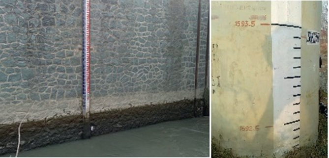
Fig. 1. Manual water level monitoring on river Jhelum
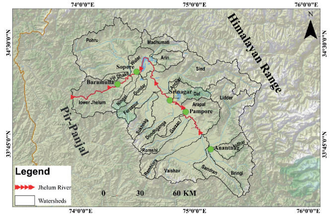
Fig. 2. Watersheds of kashmir valley with tributaries draining in river Jhelum
The daily precipitation and temperature data of 30 years ranging from 1980-2010 from three meteorological stations, Pahalgam, Kokernag and Qazigund were obtained from the India Meteorological Department. The daily water-level data from 1980-2019 of Jhelum river at three gauging stations, Sangam, Rammunshibagh, and Asham was acquired from the Department of Irrigation and Flood Control Jammu and Kashmir. The watershed of the study area was generated using the SRTM Digital Elevation Model (DEM) using ArcGIS software.
In this system, we have four base stations out of which three base stations were equipped with wireless sensors to measure different parameters and one base station namely
Sangam, where sensors are not used and data was acquired from the meteorological station. All the three WSN equipped base stations have the same architecture (Fig. 3).The system mainly depends on the wireless communication for data transmission and not on the internet because of the volatile situation of the Kashmir valley which experiences frequent internet blockade by the government for security reasons (Iqbal 2017).
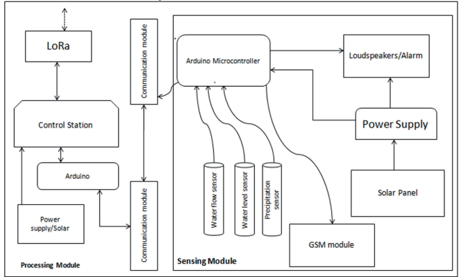
Fig. 3. Architecture of base station
The ANFIS is a multilayer feed-forward network, being so specific operations were performed on incoming signals by each node (neuron). The ANFIS is a Takagi-Sugeno model with five layers in which membership functions, inputs, and derived rules determine its structure. An optimal number of epochs (iterations in learning phase) and type of membership function determines the efficiency of the model. The ANFIS employs «if-then» rules to perform an operation(Jang 1993) which is described below for a first-order model of common two fuzzy rules (Younes et al. 2015).
Rule 1: If X1 is A1 and x2 is B1 then f =p1x1+q1x2+r1
Rule 2: if X1 is A2 and X2 is B2 then f2 =p2x1+q2x2+r2
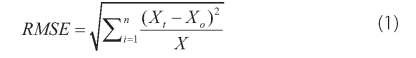
Where A and B denote grade like «Low» or «Less» whereas p1,q1,p2,q2 are parameters. The Root Mean Square Error (RMSE), Mean Absolute Error (MAE) and Coefficient of Determination (R2) statistical methods were used to evaluate the performance of the model (Antanasijevi et al. 2013).
The first and foremost thing is to select the optimal variables, which are admissible to the desired output. 120 tests were done to get the optimal number of inputs and based on these tests, the best number of inputs turned out to be four. Furthermore, the best type of membership function was determined by testing all eight types of membership functions and the hybrid type of training algorithm was used. The epoch number and membership function number was kept constant at 40 and 3 respectively. The Triangular membership function showed the best results when compared to the other membership functions as shown in table 2. This model was selected for further modification in order to enhance its performance. To finalize the best performing structure of the model, it was necessary to determine the optimum number of functions. The number of membership functions were varied from 3-6 and the epochs were kept constant at 40. The tests revealed that the optimum number of membership functions is four. The best performing membership function was selected on the basis of the smallest RMSE for training and testing.
Table 2. Membership functions with respective test values
Function Type | RMSEtrain | RMSEtest | MAEtrain | MAEtest | R-sqtrain | R-sqtest |
|---|---|---|---|---|---|---|
triangular Membership function (trimf) | 2.1357 | 3.3613 | 0.286 | 0.561 | 0.997 | 0.993 |
trapezoidal membership function (trapmf) | 2.2750 | 3.6257 | 0.317 | 0.601 | 0.991 | 0.987 |
generalized bell membership function (gbellmf) | 2.1485 | 7.4029 | 0.292 | 1.013 | 0.963 | 0.959 |
gaussian membership function (gaussmf) | 2.1556 | 4.2192 | 0.307 | 0.843 | 0.981 | 0.976 |
gaussian combination membership function (gauss2mf) | 2.2727 | 4.5048 | 0.319 | 0.775 | 0.978 | 0.969 |
pi-shaped membership function (pimf) | 2.3343 | 3.8190 | 0.395 | 0.741 | 0.981 | 0.975 |
Difference between two sigmoidal membership functions (dsigmf) | 2.2188 | 7.9834 | 0.296 | 1.107 | 0.985 | 0.905 |
Product of two sigmoidal membership functions (psigmf) | 2.2201 | 7.8919 | 0.399 | 1.091 | 0.957 | 0.893 |
The process of flood monitoring and early warning starts from the sensing module. The CS475A radar sensor is ideal for outdoor rough condition, calculates the distance between the sensor and the water by measuring the elapsed time between the emission and return of pulses. This data along with the data from rain measuring, tipping, self-emptying bucket, temperature sensor, and the magnetic hall-effect water-flow sensor is transmitted to the microcontroller. The Arduino 2560, which has 54 digital I/O pins with Atmega 2560 microcontroller sends the sensor data to the processing module of the base station via the HC-12 communication module, which is processed and a localised prediction about the future water level at this base station is made by finding a correlation between the rainfall and the water level.
Where L is the river water level, Q is the lag time, R is the rainfall, and α is the coefficient, which illustrates the correlation between water level and rainfall. The increase in the water level is directly proportional to the intensity of the rain. The data acquired through sensors is transmitted to the control center via the SX1272LoRa module. At the control center, the data is received by another SX1272 LoRa module and stored in the database. This data is later used to update the database and retrain the model. For the accurate water level prediction, the system makes use of weather forecasts from IMD (Indian Meteorological Department). The trained ANFIS model at the control center takes the forecasted values as inputs and produces an output which is the predicted value of the water level at Sangam. As we have from hourly to day to day forecasts available so this model can predict the water levels accordingly. Now, as the water level prediction for Sangam, Kakapora, Pampore and Ram munshibagh are available, The Multiple Linear Regression model takes these four predicted values as input and generates the future water level of Ram munshibagh as output which can be denoted by the equation:
Where B4 is the response variable, βi are the coefficients, where i= 0, 1, 2 and 3 are regression coefficients. B1, B2, and B3 are independent variables. The summary of the model is shown in table 3.
Table 3. Summary of LMR model
S | R-sq | R-sq(adj) | R-sq(pred) |
|---|---|---|---|
0.180179 | 98.82% | 98.78% | 98.68% |
Then this predicted water level is compared against the five warning levels which are shown in Table 3 to determine the intensity and possibility of a flood. The intervals between the data acquisition from sensors depend upon the intensity of rain and the water level. The interval of per data acquisition from sensors starts from 15 minutes, which decreases with an increase in every warning level which is shown in (eqn. 7).
Tj = Tj - ki (7)
Where Tj is the time interval between the two consecutive measurements, Δtis the increment unit, be ki ∈ {0, 1, 2, 3, 4, and 5} is the warning level. This equation means the interval between the two measurements decreases as the warning level increases. Therefore, we will have predictions that are more accurate.
Our system has five warning levels viz. Normal, High, Very High, Critical, and Flood. The time intervals of these warning levels are shown in Table 4.
Table 4. Warning levels and corresponding time intervals
Level 1 | Level 2 | Level 3 | Level 4 | Level 5 |
|---|---|---|---|---|
Normal | High | Very High | Critical | Flood |
15 Minutes | 10 minutes | 5 minutes | 1 minute | 1minute |
The proposed system was used to predict the water levels of river Jhelum at Srinagar. The ANFIS model was used to predict water level at Sangam or base station B1 because all the data was available to develop the model. The developed model has 256 rules, four-member functions for each input parameter and one output function. The efficiency of the ANFIS was evaluated using RMSE, MAE and R2 tests. The model achieved RMSEtrain (0.4306), RMSEtest (0.6109), MAEtrain (0.0623), MAEtest (0.0783), R2train (0.972) and R2test (0.966). These results were achieved at epoch number 230 and increasing epochs after that did not show any improvement in the model. The model showed that the predicted values and the measured values were almost equal with residuals falling between ±1 which signifies the efficiency of the model.The results were accurate with an accuracy of 93.53% for daily predictions and 99.91% for hourly predictions (Fig. 5, 6)

Fig. 4. Flowchart of The Proposed system

Fig. 5. Hourly Prediction Results
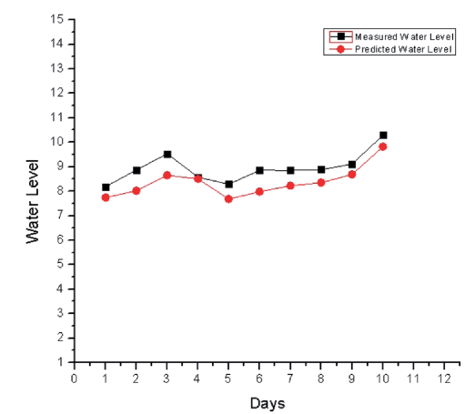
Fig. 6. Daily Prediction Results for 12 Days
The accuracy of the system in short-term predictions is better than the long-term predictions. The accuracy of the system depends on the accuracy of forecasted values of the precipitation and temperature.
In our regression model The R-sq is the regression coefficient, which determines how well the model fits our data (Dar 2018) and 98.82% is quite acceptable in our scenario (Table 5). The Adjusted R-sq value fuses the number of indicators in the model to enable you to pick the right model. The difference in the R-sq and Adjusted R-sq value for a predictor shows the contribution of that predictor in improving the model. A model with higher predicted R2 values has better prediction ability and in our case 98.68% is excellent. Usually, 0.05 significance level works well but, in our model, we got the P-value of 0.038, 0.015, 0.014, 0.008 this signify that the association between response and each term is statistically significant. The Variance Inflation Factor of 3.36, 3.39, and 4.27 for respective variables is moderate inflation of variance of a coefficient due to correlation among the predictors in our model. The acceptable range is 10 and the regression coefficient is poorly estimated if the VIF value is greater than 10 (Babin & Anderson 2014).
Table 5. Coefficients of Regression model
Term | Coef | SE Coef | T-Value | P-Value | VIF |
|---|---|---|---|---|---|
Constant | 1.771 | 0.215 | 8.24 | 0.038 |
|
B1 | 0.0448 | 0.0228 | 20.35 | 0.015 | 3.36 |
B2 | 0.1440 | 0.0791 | 22.57 | 0.014 | 3.39 |
B3 | 0.9260 | 0.0241 | 38.35 | 0.008 | 4.27 |
In Fig. 6, The probability plot of residuals approximately follows a straight line with the least number of outliers. The residuals versus fits plot verify that there is no recognizable pattern in the points and the residuals are randomly distributed and fall randomly on both sides of 0 (Fig. 7). For all observations, the distribution of residuals is shown by the histogram of the residuals and which shows only two outliers. The order in which data were collected is displayed by the residuals versus order plot. No trends or patterns are shown in residuals and thus indicating that there is no correlation between independent variables.
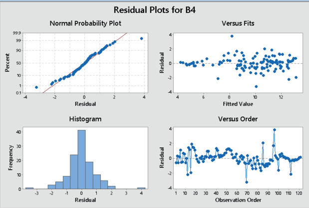
Fig. 7. Residual Plots
The system will have a direct effect on the resilience index of the valley and will contribute to the economy of the valley. As the system will provide lead time in flood warning which can be used in evacuation. This will lead to saving of many human lives; livestock and valuables. The system uses wireless sensors to measure the different factors contributing to the floods. Machine learning methods used the data to predict the possible water level. The system uses two machine learning models and wireless sensor network to perform the task of river monitoring and early flood warning. This hybrid approach paves the way to look into more possible and efficient hybrid methods to predict the various aspects and behaviors of this river under certain circumstances. The proposed system is the first Early Flood Warning system devised for Jhelum basin and covers 52.3 km of Jhelum basin from Sangam village of Anantnag district to Ram munshibagh (Srinagar). In the future, we will integrate remote sensing and GIS with machine learning methods to cover the whole Jhelum basin in Kashmir from Anantnag to Baramulla district. We can use satellite-derived rainfall (Mishra & Rafiq 2017a) temperature (Rafiq et al. 2012) and other datasets (Mishra & Rafiq 2017b) to estimate runoff and develop a sophisticated, multi-dimension early warning system. To cover the whole Jhelum basin in Kashmir we have to find some cost-effective alternatives in hardware and communication between nodes for such a long basin would be a challenging task.
1. Ahern M., Kovats R.S., Wilkinson P., Few R. & Matthies, F. (2005). Global Health Impacts of Floods : Epidemiologic Evidence. Epidemiologic Reviews (27), 36-46, DOI: 10.1093/epirev/mxi004.
2. Antanasijevi D.Z., Pocaj V.V., Povrenovi D.S., Risti M. Đ. & Peri A.A. (2013). PM 10 emission forecasting using artificial neural networks and genetic algorithm input variable optimization. Science of the Total Environment, (443), 511-519, DOI: 10.1016/j.scitotenv.2012.10.110.
3. Ashrit R. (2010). Investigating the Leh ‘cloudburst’. National Centre for Medium Range Weather Forecasting. Ministry of Earth Sciences, India.
4. Basha E. & Rus D. (2007). Design of Early Warning Flood Detection Systems for Developing Countries. Information and Communication Technologies and Development. ICTD 2007, 1-10, DOI: 10.1109/ICTD.2007.4937387.
5. Berz G., Kron W., Loster T., Rauch E. & Schimetschek J., Schmieder J., Siebert A., Smolka A., Wirtz A. (2001). World Map of Natural Hazards – A Global View of the Distribution and Intensity of Significant Exposures. Natural Hazards, (23), 443-465.
6. Bhatt C.M., Rao G.S., Farooq M., Manjusree P., Shukla A., Sharma S.V.S.P., Dadhwal V.K. (2017). Satellite-based assessment of the catastrophic Jhelum floods of September 2014, Jammu & Kashmir, India. Geomatics, Natural Hazards and Risk, 8(2), 309-327, DOI:10.1080/19475705.2016.1218943.
7. Bhatt C.M., Srinivasa Rao G., Manjushree P. & Bhanumurthy V. (2010). Space based disaster management of 2008 Kosi floods, North Bihar, India. Journal of the Indian Society of Remote Sensing, 38(1), 99-108, DOI: 10.1007/s12524-010-0015-9.
8. Cavallo E. and Noy I. (2011) Natural Disasters and the Economy – A Survey. International Review of Environmental and Resource Economics, (5), 63-102, DOI: 10.1561/101.00000039.
9. Chandran R., Ramakrishnan D., Chowdary V., Jeyaram A. & Jha A. (2006). Flood mapping and analysis using air-borne synthetic aperture radar: A case study of July 2004 flood in Baghmati river basin, Bihar. Current Science, 90(2), 249-256.
10. Dar A.A. and Anuradha N. (2018). An Application of Taguchi L9 Method in Black Scholes Model for European Call Option, International Journal of Entrepreneurship, 22(1), 1-13.
11. Do H.N., Vo M., Tran V., Tan P.V. and Trinh C.V. (2015). An early flood detection system using mobile networks. In 2015 international conference on advanced technologies for communications (ATC), 599-603. IEEE.
12. Guha-sapir D., Hoyois P. and Below R. (2017). Annual Disaster Statistical Review 2016: The numbers and trends. Review Literature And Arts Of The Americas, 1-50, DOI: 10.1093/rof/rfs003.
13. IPCC. (2001). Third Assessment Report (TAR) of the Intergovernmental Panel on Climate Change, Parts 1, 2 and 3, Cambridge University Press, Cambridge, UK. (1, 2, 3).
14. IPCC. (2014). Climate Change 2014 Impacts, Adaptation, and Vulnerability Part B: Regional Aspects, Cambridge University Press, Cambridge, UK.
15. Iqbal M. (2017). Ethnographers Lens Reviews Life in a Conflict Zone Kashmir. International Journal of Research Culture Society, 1(8) 80-86.
16. Islam A., Islam T., Syrus M.A. and Ahmed N. (2014). Implementation of Flash Flood Monitoring System Based on Wireless Sensor Network in Bangladesh, 3rd International Conference on Informatics, Electronics & Vision 2014.
17. Jang J.R. (1993). ANFIS : Adaptive-Network-Based Fuzzy Inference System. IEEE transactions on systems, man, and cybernetics, 23(3), 665-685.
18. Joseph F., Hair Jr., William C. Black, Babin B.J. and Anderson R.E. (2014). Multivariate Data Analysis, 7th ed. Pearson education limited, Eidenburgh gate, Harlow.
19. Mathur D.K. (2019). Application of Geospatial technologies in flood vulnerability analysis. Disaster Advances, 12(12), 40-45.
20. Kansal M.L., Kumar P. and Kishore K.A. (2016). Need of Integrated Flood Risk Management (IFRM) in Bihar. In National conference on Water Resources and Flood Management with special reference to Flood Modelling (WRFM-2016), Surat.
21. Kaur A., Ghawana T. and Kumar N. (2019). Preliminary Analysis of Flood Disaster 2017 in Bihar and Mitigation Measures. In Proceedings of International Conference on Remote Sensing for Disaster Management, 455-464.
22. Kim S., Kim J. & Park K. (2009). Neural Networks Models for the Flood Forecasting and Disaster Prevention System in the Small Catchment. Disaster Advances, 2(3), 51-63.
23. Kiran K.S., Manjusree P. & Viswanadham M. (2019). Sentinel-1 SAR Data Preparation for Extraction of Flood Footprints-A Case Study. Disaster Advances, 12(12), 10-20.
24. Kumar S., Sahdeo A. and Guleria S. (2013). Bihar Floods 2007: A Field Report. National Institute of Disaster Management, Ministry of Home Affairs, Government of India, New Delhi.
25. Mcbean G. (2002). Climate Change and Extreme Weather : A Basis for Action, Natural Hazards, 31, 177-190.
26. Mishra A.K., Chandra S., Rafiq M., Sivarajan N. and Santhanam K. (2016). An observational study of the Kanchipuram flood during the northeast monsoon season in 2015,Weather, 9-10, DOI: 10.1002/wea.3271.
27. Mishra A.K. (2015). A study on the occurrence of flood events over Jammu and Kashmir during September 2014 using satellite remote sensing. Natural Hazards, 78(2), 1463-1467, DOI: 10.1007/s11069-015-1768-9.
28. Mishra A. K. and Rafiq M. (2017b). Analyzing snowfall variability over two locations in Kashmir , India in the context of warming climate. Dynamics of Atmospheres and Oceans, 79 (May), 1-9, DOI: 10.1016/j.dynatmoce.2017.05.002.
29. Mishra A.K., Nagaraju V., Rafiq M. and Chandra S. (2019). Evidence of links between regional climate change and precipitation extremes over India. Weather, 74(6), 218-221.
30. Mishra A.K., Meer M.S. and Nagaraju V. (2019b). Satellite-based monitoring of recent heavy flooding over north-eastern states of India in July 2019. Natural Hazards, 97(3), 1407-1412.
31. Mishra A.K. and Rafiq M. (2019). Rainfall estimation techniques over India and adjoining oceanic regions. Current Science, (January), DOI:10.18520/cs/v116/i1/56-68.
32. Mishra A.K. and Rafiq M. (2017a). Towards combining GPM and MFG observations to monitor near real time heavy precipitation at fine scale over India and nearby oceanic regions. Dynamics of Atmospheres and Oceans, 80 (October), 62-74, DOI: 10.1016/j.dynatmoce.2017.10.001.
33. Natividad J.G. and Mendez J.M. (2018). Flood Monitoring and Early Warning System Using Ultrasonic Sensor. IOP Conference Series: Materials Science and Engineering, 325(1). DOI: 10.1088/1757-899X/325/1/012020.
34. Pal I., Singh S., and Walia A. (2013). Flood Management in Assam , INDIA : A review of Brahmaputra floods 2012. International Journal of Scientific and Reasearch Publications, 3(10), 1-5, www.ijsrp.org/research-paper-1013/ijsrp-p2214.pdf.
35. Pengel B., Shirshov G.S., Krzhizhanovskaya V.V., Melnikova N.B., Koelewijn A.R., Pyayt A.L. and Mokhov I.I. (2013). Flood early warning system: sensors and internet. Floods: From Risk to Opportunity (January), 445-453, DOI: 10.1177/1745691612459060.
36. Rafiq M. and Mishra A.K. (2016) Investigating changes in Himalayan glacier in warming environment: a case study of Kolahoi glacier. Environmental Earth Sciences. 1; 75(23):1469.
37. Rafiq M. and Mishra A.K. (2017). A study of heavy snowfall in Kashmir, India in January 2017. Weather, 99 (January), 23-25.
38. Rafiq M., Mishra A.K., Romshoo S.A. and Jalal F. (2019). Modelling Chorabari Lake outburst flood , Kedarnath , India. Journal of Mountain Science, 16 (October 2018), 64-76.
39. Rafiq M., Rashid I. and Romshoo S.A. (2012). Estimation and validation of Remotely Sensed Land Surface Temperature in Kashmir Valley. Journal of Himalayan Ecology & Sustainable Development, 9, 1-13.
40. Rezaeianzadeh M., Tabari H., Yazdi A.A., Isik S. & Kalin L. (2013). Flood flow forecasting using ANN, ANFIS and regression models. Neural Computing and Applications, 25(1), 25-37, DOI: 10.1007/s00521-013-1443-6.
41. Romshoo S.A., Altaf S., Rashid I., Dar R.A. (2018). Climatic, geomorphic and anthropogenic drivers of the 2014 extreme flooding in the Jhelum basin of,of Kashmir, India. Geomatics, Natural Hazards and Risk, 9(1), 224-248.
42. Roy J.K., Gupta D. & Goswami S. (2012). An improved flood warning system using WSN and artificial neural network. 2012 Annual IEEE India Conference, (INDICON 2012), (December), 770-774, DOI: 10.1109/INDCON.2012.6420720.
43. Singh Y., Deep K. and Niranjan S. (2012). Multiple Criteria Clustering of Mobile Agents in WSN,International Journal of Wireless & Mobile Networks , 4(3), 183-193.
44. Singh O. and Kumar M. (2013). Flood events, fatalities and damages in India from 1978 to 2006. Natural Hazards, 69, 1815-1834, DOI: 10.1007/s11069-013-0781-0.
45. Seenirajan M., Natarajan M., Thangaraj R. and Bagyaraj M. (2017) Study and Analysis of Chennai Flood 2015 Using GIS and Multicriteria Technique. Journal of Geographic Information System, 9, 126-140, DOI: 10.4236/jgis.2017.92009.
46. Sunkpho J. and Ootamakorn C. (2011). Real-time flood monitoring and warning system. Songklanakarin Journal of Science and Technology, 33(2), 227-235, DOI: 10.1016/s0959-8049(11)72694-6.
47. Thayyen R.J., Dimri A.P., Kumar P. and Agnihotri G. (2013). Study of cloudburst and flash floods around Leh, India, during August 4-6, 2010. Natural Hazards, 65(3), 2175-2204, DOI: 10.1007/s11069-012-0464-2.
48. Younes M.K., Nopiah Z.M., Basri N.E.A., Basri H., Abushammala F.M., Maulud K.N.A. and Maulud K.N.A. (2015). Solid waste forecasting using modified ANFIS modeling. Journal of the Air & Waste Management Association, 65(10), 1229-1238, DOI: 10.1080/10962247.2015.1075919.
Department of Computer Applications
Vandalur Ch-600048
Department of Computer Applications
Vandalur Ch-600048
Imran M., P. Sheikh A. Forecasting Water Level Of Jhelum River Of Kashmir Valley India, Using Prediction And Earlywarning System. GEOGRAPHY, ENVIRONMENT, SUSTAINABILITY. 2020;13(2):35-42. https://doi.org/10.24057/2071-9388-2019-169

Editor-in-Chief
Kasimov Nikolay S.Lomonosov Moscow State University
Moscow 119991 Russia, Leninskie Gory, Faculty of Geography, 1806a
Phone +7 495 939-15-52
Fax: + 7 495 939-15-52
E-mail: ges-journal@geogr.msu.ru


